Example workflow

modality XPLR workflows utilise data generated by duet software, to run statistical analysis and explore methylation patterns across the 6-base genome. A genome annotation can be used to examine the context of differences in methylation, providing mechanistic insight into the dynamic nature of methylation changes. modality XPLR consists of modular steps allowing an analysis flow to be built to address specific biological questions.

In this worked example, we are using a colorectal cancer (CRC) dataset of liquid biopsy samples (cfDNA) to demonstrate a typical discovery workflow. We will use the workflow to determine the methylation status of promoters at different stages of disease and investigate if discrimination of 5mC and 5hmC could provide new biomarkers for earlier stage disease.

Overview of the workflow

The workflow steps:

• Summarise Zarrs, confirm the depth of CpG coverage, and ask whether methylation patterns make biological sense, according to the experimental design, using modality biological-qc.

• Assess depth and coverage in specific regions of interest, e.g. gene promoters using modality get mean.

• Identify 5mC DMRs in promoter regions between Healthy Controls and Stage IV disease cfDNA using modality dmr call.

• View DMR results in a volcano plot, apply filters and identify regions with significant hypo-methylation in Stage IV cfDNA compared to Healthy Controls, using modality dmr plot.

• Using significantly hypo-methylated 5mC DMRs from the previous step as a biological prior, identify 5hmC DMRs between Healthy Controls and Stage I disease cfDNA using modality dmr call.

• View 5hmC DMRs in a volcano plot to identify promoter regions with significant hyper-methylation in Stage I cfDNA compared to Healthy Controls, using modality dmr plot, as a potential biomarker for early stage disease.

• Bring the analyses together to visualise the methylation changes in biological context, by aligning the results with genome annotations using modality tracks.

• Generate a set of 5mC and 5hmC features that can be used to build a model for early disease classification using modality get regional-frac for mc and hmc.

Note

When creating the workflow of modality XPLR features this example shows the iterative process, for example running DMR analysis for Controls vs Stage IV samples, and then using the DMR results .bed output as an input --bedfile for DMR analysis of Controls vs Stage I samples.

Let’s examine each of these steps in this worked example, with a note to cover why the step is included, what inputs are needed, the commands used, and the outputs available for immediate results or for the next step of the workflow.

1. Assess methylation data quality

The first step is to ensure there is enough coverage for meaningful onwards statistical analysis, and assess whether expected methylation patterns are present, based on the experimental question. This is done with modality biological-qc

Insights gained from running Biological QC:

What does the analysis tell us?	Using which visual?
Confirmation that mean CpG coverage is sufficient for downstream analyses.	Summary table
Whether methylation levels of similar or different samples follow anticipated correlations e.g. replicates are similar, different disease stage samples show different levels of correlation.	Pearson correlation matrix
Samples cluster with expected ‘like’ samples e.g. controls, stage of disease and the feature on axis is significant in the analysis e.g. level of 5mC or 5hmC etc. and identification of outliers.	PCA scatterplot

Inputs

• Zarr store(s): Paths to each Zarr store to include in the analysis.

• Sample sheet (recommended): Path to the sample sheet file containing metadata about the samples.

• Output directory (recommended): Path to the output directory where the HTML report will be saved.

Example code

When modality biological-qc is invoked, all three analyses above run automatically and are presented in a single HTML report.

modality biological-qc \
        --zarr-path path/to/data.zarrz \
        --sample-sheet path/to/sample_sheet.csv \
        --aggregate-by-group "label" \
        --disable-strand-merging \
        --region chr1 \
        --output-dir path/to/output/directory

Example outputs including plots

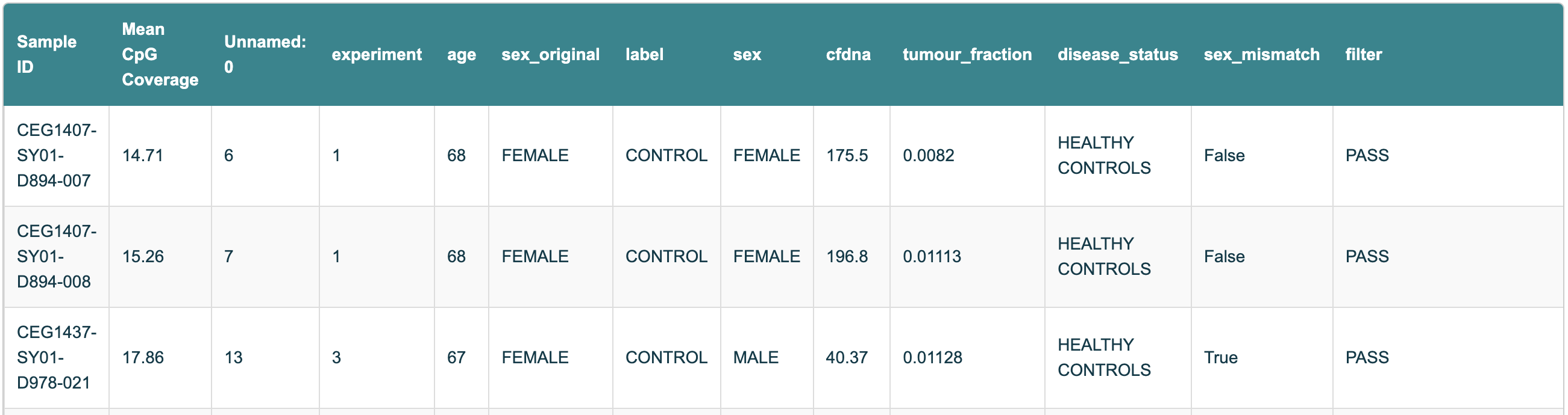
Figure 10 Snapshot of the Sample Information table from the Biological QC HTML report, showing Sample IDs and the corresponding mean CpG coverage.

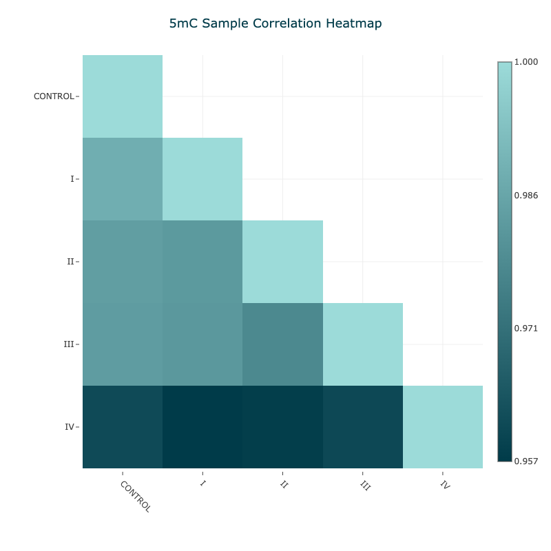
Figure 11 5mC Pearson correlation matrix for aggregated samples

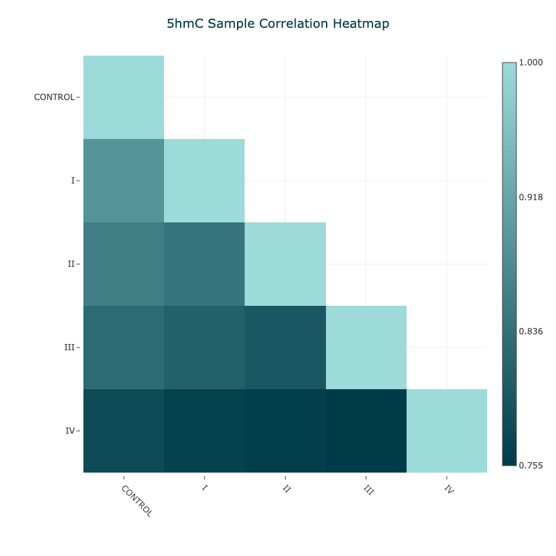
Figure 12 5hmC Pearson correlation matrix for aggregated samples

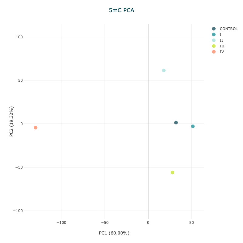
Figure 13 5mC PCA plot showing aggregated samples by disease stage

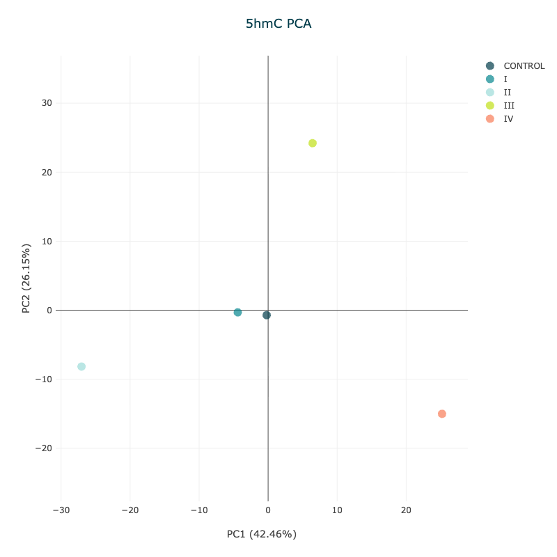
Figure 14 5hmC PCA plot showing aggregated samples by disease stage

2. Checking CpG context depth across the regions of interest

In step 1, the summary table reports the general sequence coverage across all the samples. Let’s look at how adding modality get analysis at this stage helps to check the coverage is sufficient at the specified promoter regions of interest.

Note

A prep-prepared bedfile of annotated promoter regions is used to focus on the regions of interest, see Pre-prepared BED files.

What is being analysed?	Subcommand	Output
The mean coverage of CpGs per region of interest.	modality get mean	A violin plot of coverage per region of interest
The number of CpGs per region of interest, with coverage ≥10	modality get count	A table of counts per region of interest (TSV file)

Inputs

• Zarr path: Path to the Zarr file(s) containing methylation data.

• Fields: Type(s) of cytosine to extract, which in this example is total_c (mc + hmc + c).

• Region definition: Path to a BED file defining the promoter sites as the regions of interest.

• Minimum coverage: When applicable, the level of coverage at a CpG site needed to be included in the analysis.

• Output directory: Path to the output directory where the results of the analysis will be saved.

Example code and outputs

First, to view the coverage distribution of CpGs at promoter regions, we can use the modality get mean command. The violin plot is included in the output HTML report.

modality get mean \
        --zarr-path path/to/data.zarrz \
        --fields total_c \
        --bedfile path/to/gencode.v44.human.promoters.annotation.tsv \
        --disable-strand-merging \
        --output-dir path/to/output/directory

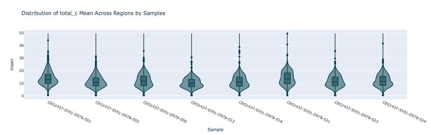
Figure 15 Violin plot showing the mean coverage of total_c per promoter region, for 8 samples.

Next, we may want to filter the promoter regions to only include those with sufficient coverage, for example, where the mean coverage is greater than 10. This can be done by first using the modality get count command, and then filtering the output .tsv to update the list of promoters for downstream processing.

Alternatively, minimum coverage settings can be applied directly in modality XPLR functions such as modality dmr call or modality get regional-frac. Note that the filter value should be selected according to whether strands are merged (default) or not (--disable-strand-merging) in the analysis. If strand merging is disabled, as shown here, the expected CpG coverage will be approximately half the NGS depth.

modality get count \
--zarr-path path/to/data.zarrz \
--fields total_c \
--bedfile path/to/gencode.v44.human.promoters.annotation.tsv \
--min-coverage 5 \
--disable-strand-merging \
--output-dir .path/to/output/directory

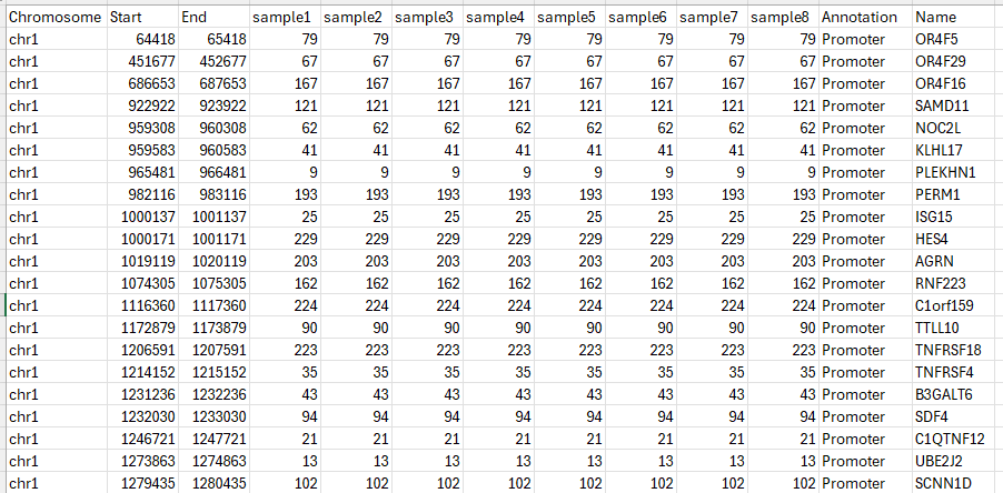
Figure 16 Snapshot of the output tsv.gz for 8 samples, showing the number of CpGs per promoter region with coverage ≥5.

3. Call differentially methylated regions (DMRs) in late stage disease

With sufficient coverage confirmed of the regions of interest, the next step is to call DMRs in late stage disease to identify promoter regions where demethylation (hypo-methylation) is observed compared to Healthy Controls.

What is being analysed?	Output
To look for biomarkers of early disease, we first establish our biological priors by looking for changes in promoter regions between Healthy Controls and late-stage (Stage IV) cfDNA. We are looking to identify changes in 5mC.	5mC DMR .bed result file for the comparison of Healthy Controls and Stage IV cfDNA samples. .ini files and provenance metadata files.

Inputs

• Sample sheet: The sample sheet is a .csv or .tsv file that contains metadata about the samples in the Zarr store.

• Zarr path: Path to the Zarr file(s) containing methylation data.

• Region definition: Path to a BED file defining the promoter sites as the regions of interest.

• Methylation context: Type(s) of cytosine to extract, which in this example is num_mc.

• Output directory (optional): Path to the output directory where the results of the analysis will be saved.

Tip

Before starting analysis care should be taken to prepare the sample sheet to ensure the correct data is used. Note the column header name(s) that refer to the sample group or condition, and covariates (if applicable).

Example code

modality dmr call \
        --sample-sheet path/to/metadata.csv \
        --condition-array-name label \
        --zarr-path path/to/data.zarrz \
        --methylation-contexts mc \
        --bedfile path/to/promoters.bed \
        --condition-order "CONTROL" "IV" \
        --output-dir path/to/output/directory \
        --min-coverage 10 \
        --overdispersion​

Note

--overdispersion was used in case the false positive occurrence was too high. This may not be necessary once the data has been examined. See Overdispersion correction in the user guide for more details.

Example outputs including plots

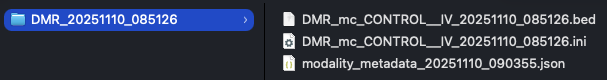
Figure 17 The output folder structure of the modality dmr call command. A timestamped sub-directory is created, containing the DMR results bedfile, provenance metadata file, and configuration .ini file.

Note the path of the DMR results bedfile, for use in modality dmr plot in the next step of the analysis.

What is being analysed?	Using which visual?
Finding samples where methylation differences are significant being either areas of hypo- or hyper-methylation	Volcano plot

Note

In this worked example the hypo-methylation regions were of interest as an indicator of where demethylation may have occurred in late stage disease. This allows us to ask whether we could detect increases of 5hmC in the same regions, at an earlier stage of disease.

Inputs

• DMR results: Path to the DMR results bedfile.

• Output directory: Path to the output directory where the results of the analysis will be saved.

Example code

modality dmr plot \
        --dmr-results path/to/DMR_mc_CONTROL__IV_20251110_085126.bed \
        --output-dir path/to/output/directory

Example outputs including plots

In differential methylation analysis, a volcano plot is a powerful visualisation tool that helps identify regions with both statistically significant and biologically meaningful differences in methylation between two groups. In the below plot we have DMRs called on 5mC comparing the two groups control and Stage IV in cfDNA data. The axes of the volcano plot represent:

• X-axis: Modification difference (e.g., methylation difference between two groups, often called \(\Delta\beta\) or \(\Delta \text{methylation}\)).

• Y-axis: Log10-transformed q-value (adjusted p-value) although note that when hovering over the data points you will see key information regarding the data point including the non-transformed q-values which is more commonly interpreted.

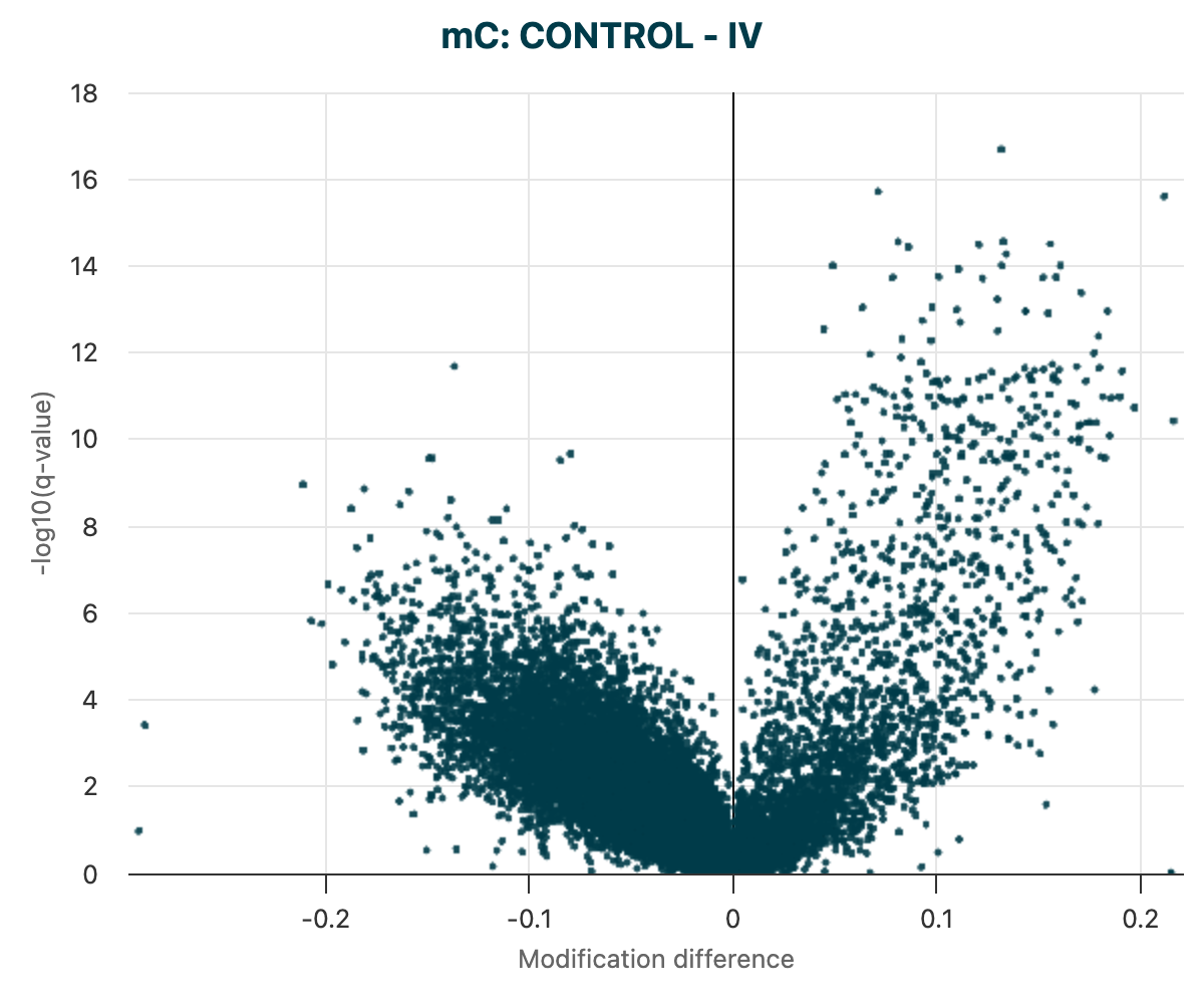
Figure 18 The unfiltered volcano plot of DMR results for 5mC DMRs, between Control vs Stage IV cfDNA samples.

4. Filtering DMRs to identify statistically significant changes

Rather than working with all regions, the next step was to identify a subset of regions with statistically significant DMRs meeting a given threshold.

What is being analysed?	Using which visual?
To speed up analysis and to focus on regions with statistically significant differences, filters are applied to create a results file with DMR calls passing a significance threshold and level of change in methylation.	Volcano plot of 5mC DMRs. Data points visible in the plot are determined by the dmr plot tool.

Inputs

• DMR result file(s): Paths to the output(s) of the modality dmr call tool, in BED3+ format.

Example code

modality dmr plot \
        --dmr-results path/to/DMR_mc_CONTROL__IV_20251110_085126.bed \
        --filter-qvalue 0.01
        --filter-mod-difference 0.15
        --output-dir path/to/output/directory

Tip

If there is a delay when interacting with the HTML plots, this could be due to having too many data points. This can be addressed by setting more stringent filters to reduce the number of data points to render.

Example outputs including plots

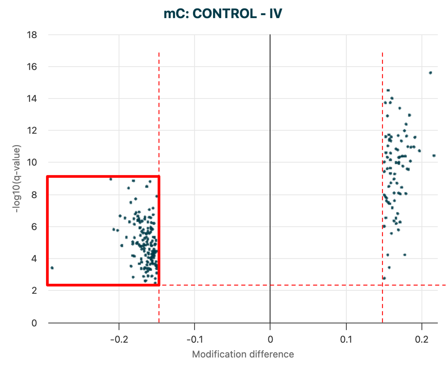
Figure 19 The filtered volcano plot of DMR results for 5mC DMRs, between Control vs Stage IV cfDNA samples.

The dmr plot command also produces a filtered results .bed file, which can be used in the next step of the analysis.

In this example, we are interested in the regions showing significant 5mC hypo-methylation at Stage IV, compared to Healthy Controls. We hypothesise that these regions will give rise to early biomarkers of change when looking at 5hmC levels, because changes in 5hmC are expected to precede the loss of 5mC.

5. Use biological priors to call DMRs in early stage disease

The previous step in the analysis identified DMRs with hypo-methylation in late stage disease. Next, we can ask if these same regions show an increase in 5hmC levels in early stage samples compared to Healthy Controls. This may reveal a biomarker of early change, where 5hmC may signal that a region is primed for later demethylation.

What is being analysed?	Using which visual?
To assess whether hypo-methylation of promoters in Stage IV samples display increase in 5hmC levels at these sites in Stage I vs Healthy Controls.	DMR calling only.

Inputs

• Filtered 5mC-DMR bedfile: Path to the output file from above.

• Sample sheet: Use the same sample sheet as used in the previous step, which contains metadata about the samples in the Zarr store.

• Zarr path: Path to the Zarr file(s) containing methylation data.

• Output directory (optional): Path to the output directory where the results of the analysis will be saved.

Example code

modality dmr call \
        --sample-sheet path/to/metadata.csv \
        --condition-array-name label \
        --zarr-path path/to/data.zarrz \
        --methylation-contexts hmc \
        --bedfile path/to/filtered_5mC-DMRs.bed \
        --condition-order "CONTROL" "I" \
        --output-dir path/to/output/directory \
        --min-coverage 10 \
        --overdispersion

Outputs

A new timestamped DMR results directory containing the DMR results file with your calls, an ini file that can be used to view your DMRs in their genomic context using the modality tracks command.

6. Visualisation of key early-stage 5hmC DMRs

Again, this step uses modality dmr plot to visualise the DMR results file generated previously (modality dmr call).

What is being analysed?	Using which visual?
Visualisation of promoter regions where DMRs show statistically significant increase in 5hmC levels at Stage I versus 5mC hypo-methylation in Stage IV allowing selection of specific regions for further investigation.	Volcano plot of 5hmC DMRs.

Inputs

• DMR results file: The DMR results file just created, focussed on the 5hmC levels in the Control and Stage I samples at the hypo-methylated promoter sites from Stage IV samples.

• Output directory: Path to the output directory where the results of the analysis will be saved.

Example code

modality dmr plot \
        --dmr-results path/to/DMR_hmc_CONTROL__I_20251109_214630.bed \
        --output-dir path/to/output/directory

Tip

If there is a delay when interacting with the HTML plots, this could be due to having too many data points. This can be addressed by setting more stringent filters to reduce the number of data points to render.

Example outputs including plots

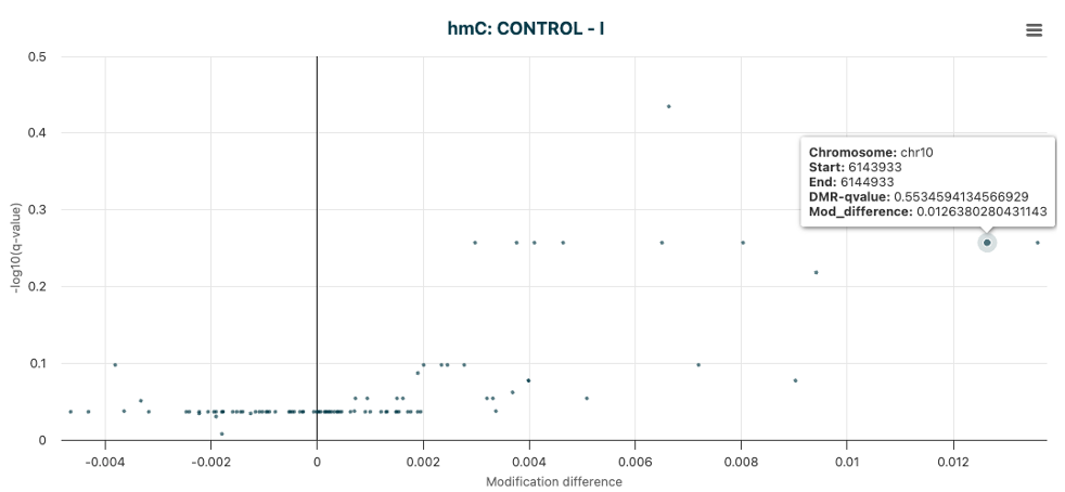
Figure 20 The unfiltered volcano plot of DMR results for 5hmC DMRs, between Control vs Stage I cfDNA samples.

From this plot, or directly from the DMR results file, we can identify regions of interest for further investigation. In this example, the promoter region of PFKFB3 was identified as a region of interest, where 5hmC levels were increased in Stage I samples compared to Controls, additional analysis showed 5mC levels were significantly decreased in Stage IV samples compared to Controls. The next step is to bring together the DMR results and genomic annotation to look at biological context of the selected regions.

7. Place methylation changes (DMRs) into genomic context

From the analysis so far, the last DMR plot will identify promoters that warrant further investigation. modality tracks allows a combined view of specific 5mC (Stage IV) and 5hmC (Stage I) DMRs by modifying the .ini configuration file, including added annotated genomic context.

In this example, we will use the promoter region of PFKFB3 as a region of interest, which was identified in the previous step. The 1000bp promoter region is defined as chr10:6143933-6144933, which we will view in a track plot with an additional 1000bp padding on either side, to allow for visualisation of the surrounding genomic context.

What is being analysed?	Using which visual?
Bringing together the DMR results and genomic annotation to place significant DMRs in biological context.	modality tracks

Inputs

• ini file: Path to the .ini file to be included in the analysis.

• Output directory: Path to the output directory where the track plot image will be saved.

Tip

For details on the default .ini file, adapting the .ini file or creating a specific .ini file, refer to the 1. Auto-generated .ini file and 2. Customising .ini files sections of the user guide.

Example code

modality tracks \
        --region chr10:6143933-6144933 \
        --padding 1000 \
        --tracks-file path/to/config.ini \
        --output path/to/output/directory/track_plot.png

Example output

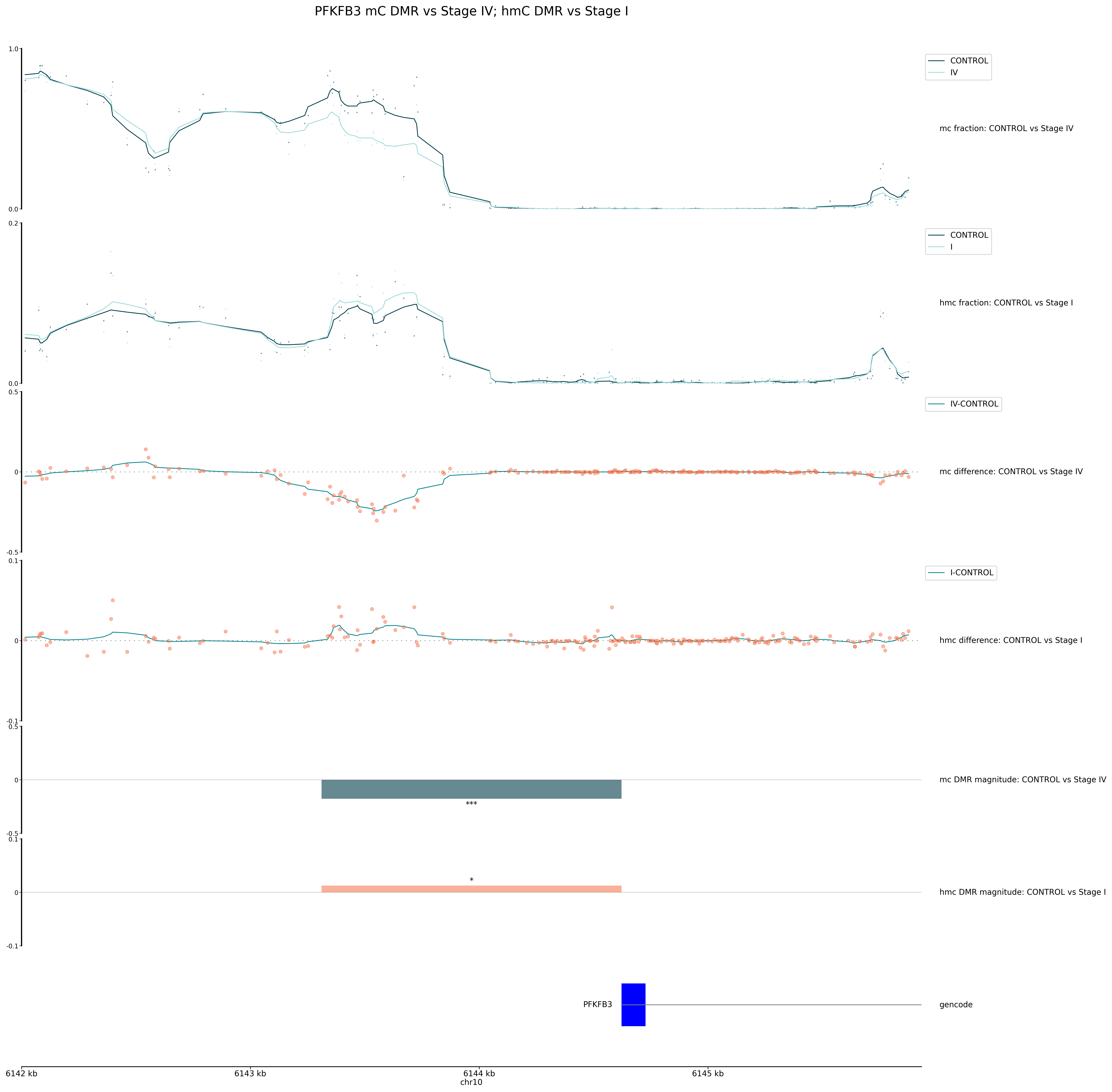
Figure 21 A combined track plot showing the methylation levels of 5mC and 5hmC in the promoter region of PFKFB3, with DMRs highlighted.

Interpreting the tracks plot:

The output file is named according to the specified path and file extension, and includes:

• Methylation traces:

  • In this example the top tracks display the 5mC and 5hmC methylation fraction for each group. The top trace shows the 5mC fraction for CONTROL and Stage IV cfDNA, and the bottom trace shows the 5hmC fraction for CONTROL and Stage I cfDNA.

  • Each line represents the average methylation fraction across the region for a group.

  • Dots indicate per-site values (e.g. CpGs).

  • These traces allow you to see overall methylation patterns and differences between groups. At DMRs, we expect to see divergence between the average methylation trace lines between groups.

  • Trace plots are drawn directly from the Zarr data with the strand merging setting used during DMR calling by default.

• Modification differences:

  • Below the methylation traces, the next tracks show the 5mC and 5hmC modification difference between groups. The first shows the 5mC modification difference for CONTROL and Stage IV cfDNA, and the second shows the 5hmC modification difference for CONTROL and Stage I cfDNA.

  • The y-axis represents the difference in methylation fraction between the two groups at each position.

  • Points show raw differences and lines show smoothed differences, highlighting regions of gain or loss.

  • This helps to quantify the relative difference of methylation changes between groups. Note the difference in y-axis scale between the two tracks, as the 5mC hypo-methylation in Stage IV is much greater than the 5hmC hyper-methylation in Stage I.

• DMR tracks:

  • The next panels highlight the locations and magnitude of DMRs. The length and position of the bars will match the specified window size or defined regions used as input to DMR calling.

  • Bar colour and height reflect the direction and magnitude of change (e.g., hypo-methylation or hyper-methylation). For example, a blue bar may indicate a region of significant 5mC loss in Stage IV, while a red bar may indicate a region of 5hmC gain in Stage I.

  • The number of asterisks above each bar, describes the level of statistical significance, where:

    • One asterisk (*) indicates a q-value < 0.05

    • Two asterisks (**) indicate a q-value < 0.01

    • Three asterisks (***) indicate a q-value < 0.001

    • Note: If a q-value is not listed in the DMR results file, the asterisks will be based on the p-value, with the same significance levels as above.

• Annotations:

  • At the bottom, the gene annotation track shows the genomic features in the displayed region.

  • This track is based on the GTF/GFF3 file specified in the .ini file.

  • In this example, genes are displayed with exons as blue boxes, and labels (e.g., “PFKFB3”) for easy identification.

  • This context allows you to relate methylation changes to known genes or regulatory elements, supporting biological interpretation. We can see that the DMR block matches the 1000bp region upstream of the gene TSS, denoted as a promoter region in the DMR input bedfile.

8. Generate feature sets for building classifiers

Using the methods described above, it is possible to generate feature sets that can be used to build classification models. This can be achieved by extracting different statistical measures for 5mC and 5hmC for your regions of interest. In this case we will be extracting the regional fractions for the regions provided in --bedfile with modality get regional-frac.

What is being analysed?	Output
The fraction of 5mC in the regions of interest (the promoter regions)	.tsv files and HTML report containing violin and correlation plots.
The fraction of 5hmC in the regions of interest (the promoter regions)	.tsv files and HTML report containing violin and correlation plots.
[Optional] Co-methylation and clustering analysis of 5mC and 5hmC fractions across a specific subset of regions, e.g informed by gene ontology data.	Additional regional heatmap included in the HTML report, for up to 200 regions.

Inputs

• Zarr Path: Path to the Zarr file(s) containing methylation data.

• fields: The types of cytosine to extract; in this example both mc and hmc.

• Region Definition: Path to a .bed file defining the promoter sites as the regions of interest.

• Output directory: Path to the output directory where the result files will be saved.

Example code

To generate regional fraction for both 5mC and 5hmC accross a broad set of regions (e.g. all promoters), the following command can be used:

modality get regional-frac \
        --zarr-path path/to/data.zarrz \
        --fields mc hmc \
        --bedfile path/to/gencode.v44.human.promoters.annotation.tsv \
        --min-coverage 10 \
        --disable-strand-merging \
        --output-dir path/to/output/directory

To generate regional fraction for a smaller set of regions (e.g. gene pathways), the same command can be used with a different --bedfile input and --heatmap options. Including a metadata sample sheet allows control for which samples to include.

modality get regional-frac \
        --zarr-path path/to/data.zarrz \
        --sample-sheet path/to/metadata.csv \
        --order-by-group label \
        --fields mc hmc \
        --bedfile path/to/gene-region-subset.bed \
        --min-coverage 10 \
        --disable-strand-merging \
        --heatmap \
        --output-dir path/to/output/directory

Example data output

Figure 22 Snapshot of an output tsv.gz for 8 samples, showing the 5hmC fraction per region, with a depth ≥10. Rows with no data indicate that the region/sample did not meet the --min-coverage requirement. Regions with “0” fraction indicate that CpGs were covered, but no methylation was detected in that region for that methylation context (e.g., 5hmC).

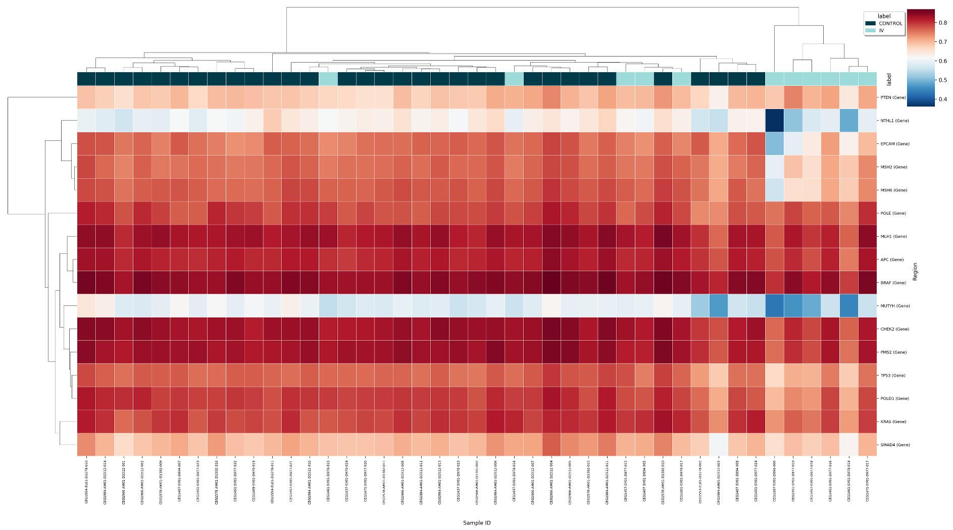
Figure 23 Regional co-methylation heatmap for 5mC enrichment in Control and Stage IV samples, for 16 gene regions implicated in CRC.

Conclusion

This worked example has shown how to use modality XPLR to run a series of analyses on methylation data, starting from quality control and coverage checks, through to identifying DMRs and visualising them in biological context. The steps outlined above demonstrate how to build a workflow using modality XPLR to address a specific biological question, in this case, the investigation of methylation changes in promoter regions across different stages of disease. The final step of the workflow is to extract features from the DMRs identified, which can be used to build classification models for potential biomarkers. This example highlights the modular nature of modality XPLR, allowing analyses to be tailored to specific needs and biological questions.

Note

This example is intended to provide a general overview of how to use modality XPLR for methylation analysis. The specific commands and parameters may vary depending on the dataset and research question. It is recommended to refer to the modality XPLR user guide for detailed information on each command and its options.

For further information about the utility of 5mC and 5hmC as biomarkers for early disease detection, refer to our recent publication on BioRxiv:

5-methylcytosine and 5-hydroxymethylcytosine are synergistic biomarkers for early detection of colorectal cancer