Toolkit

Preparing for analysis

Input file types

modality XPLR offers a variety of analysis workflows, that leverage common input files and parameters.

The main input files are described in this section, and include:

• Zarr store files, .zarrz

• Sample sheet, .csv or .tsv

• Region files in BED3+ format, .bed or .tsv

Input files from external sources may be required, such as annotation references (.gtf or .gff). Descriptions of these file types and formats are also provided below.

Zarr store

The Zarr store is a compressed file format (.zarrz) used to store large datasets in a distributed manner. It is designed for efficient storage and retrieval of large arrays, making it suitable for high-throughput sequencing data such as methylation data. The Zarr format allows for chunked storage, enabling efficient access to subsets of data without loading the entire dataset into memory. This is particularly useful for large datasets that may not fit into memory all at once.

The Zarr store is a directory structure that contains metadata and data files. The metadata files describe the structure and properties of the dataset, while the data files contain the actual data. The Zarr store can be accessed using various programming languages and tools, including Python, R, and command-line interfaces.

In the context of modality XPLR, the Zarr store contains methylation count data for one of the cytosine contexts: CpG, CHG, or CHH. By default, the upstream duet pipeline generates CpG context data, but it can be configured to produce CHG or CHH context data as well. Each Zarr store contains data for only one context type at a time. For each site in the selected context, the Zarr store records the number of modified cytosines (5-methylcytosine and 5-hydroxymethylcytosine for duet evoC, modified cytosines for duet +modC) and unmodified cytosines, as identified in base-resolution sequencing data, along with total coverage and related counts (see table below for a full list).

For biomodal workflows, the Zarr store containing methylation data is produced by the upstream duet software. You will need the path to each Zarr store for your dataset to run the modality XPLR software. For simplified management, Zarr stores can be combined. See the section for Handling Zarr stores and the modality zarr-utils join operation for more information.

A list of count data variables contained in the Zarr store is provided below:

Data variable	Description
c	Unmodified C’s.
mc	5-Methylcytosine (5mC) present in 6-base Zarr
hmc	5-Hydroxymethylcytosine (5hmC) present in 6-base Zarr.
modc	Combined 5mC and 5hmC signal (modC).
total_c	Total number of modified and unmodified C’s (mc + hmc + c).
total	Sum of total_c + n + other (where n is an unresolved base).
other	SNPs in CpGs, i.e. where the CpG base is not a c or n.

Sample sheet

The sample sheet is a .csv or .tsv file that contains metadata about the samples in the Zarr store. The sample sheet can be created using any text editor. It must be saved as a .csv or .tsv file with the header row included. The sample sheet must include a column header, sample_ids, listing one or more sample IDs that match the sample IDs in the Zarr store. The sample sheet can also include additional columns with metadata, such as grouping information (e.g., sample type, condition), or covariates (e.g., age, smoker status, batch information). The analysis operations can handle both continuous and categorical metadata.

Formatting the sample sheet

modality XPLR expects UTF-8 encoding for sample sheet files but is fully compatible with ASCII characters. Do not use non-ASCII (Unicode) characters. Avoid using special characters, spaces, or commas in the sample sheet. We recommend using underscores (_) instead of spaces in the sample IDs and column headers. If you edit the sample sheet in a text editor, ensure it is saved as plain .csv or .tsv and that no extra spaces or formatting are introduced.

• Column Headers

  • Column headers must not contain spaces or commas.

  • Use only ASCII letters, numbers, and underscores (_) in column headers.

  • Each column header must be unique.

  • The first column must be named sample_id (case-sensitive) and contain unique sample identifiers.

  • Additional columns can be used for grouping (e.g., disease_stage) or covariates (e.g., age, smoker_status).

• Sample IDs

  • Sample IDs must not contain spaces or commas.

  • Use only ASCII letters, numbers, and underscores (_) in sample IDs.

  • Each sample ID must be unique within the sample sheet.

  • Sample IDs must exactly match those used in the Zarr store(s).

Important

Sample sheet metadata can be used for grouping samples in the analysis. Ensure that one of your columns can be used to group samples to use the grouping functions for Biological QC, DMR calling and Feature Extraction.

The sample sheet should be formatted as follows:

e.g., Sample IDs to be grouped by disease_stage, with the covariate smoker_status included in the analysis.

sample_id	disease_stage	smoker_status
sample1	control	no
sample2	I	yes
sample3	I	no
sample4	IV	yes
sample5	IV	no

Define a single region

Several of the tools in the modality XPLR software allow you to specify a single region of interest for analysis. This can be done by specifying the region in the command line using the format chr or chr:<start>-<end>. The start and end positions are optional, and indices are zero-based and half-open.

For example, to specify the region on chromosome 1 from position 1000 to 2000, use the following format: chr1:1000-2000. This will restrict the analysis to a specific region of the genome, which can be useful for focusing on regions of interest or reducing the size of the dataset during analysis. The region can be specified in the command line using the --region option. For example:

modality dmr call \
   --zarr-path path/to/data.zarrz \
   --methylation-contexts mc hmc \
   --region chr1:1000-2000 \
   --output-dir path/to/output

Note

If using --region in combination with --window-size, the specified region will be divided into windows of the specified size. Similarly, you can use a bedfile format to specify individual window sizes over a larger region of interest. See the Region files section below.

Region files

The user-supplied region file is a BED3+ format (.bed or .tsv) file that contains genomic regions of interest for analysis. It should include columns for the chromosome, start position, and end position of each region. The region file is optional but can be used to restrict the analysis to specific regions of the genome. The region file should be formatted as follows:

e.g., Region file with regions of interest.

chromosome	start	end
chr1	1000	2000
chr1	3000	4000
chr2	5000	1000
chr2	7000	3000

Annotations are optional but can be included in the analysis to provide additional context and information about the genomic regions of interest. Annotations can include information such as gene names, gene symbols, gene biotypes, and other relevant features. The annotations must be included in the region file and should be formatted as follows:

e.g., Region file with annotations.

chromosome	start	end	annotation	name
chr4	25250935	25251935	Promoter	KRAS
chr5	112706517	112707517	Promoter	APC
chr17	7687537	7688537	Promoter	TP53

Note

A region file can contain multiple different annotation classes, such as promoters, enhancers, or other genomic features.

Preparing annotation files

There are two types of annotation files that are used in the modality XPLR software:

• Annotated region files: Used to define genomic regions for analysis. E.g. as input to the modality dmr call and modality get tools.

• Genome annotation GTF/GFF3 files: Used to annotate new region definitions with modality prepare-regions (GFF3) or to place analysis outputs into a broader biological context with the modality tracks (GTF) tool.

You can download the human hg38 GENCODE v44 annotation files for the human (hg38) genome from biomodal, or prepare your own annotation files from public databases as described below.

To access biomodal demo data resouces, you need to install gcloud CLI and authenticate. See the download instructions here then use the following command:

gcloud storage cp gs://biomodal-data/annotation/gencode.v44.basic.annotation.gff3.gz .

gcloud storage cp gs://biomodal-data/annotation/gencode.v44.annotation.gtf.gz .

Alternatively, annotation files can be downloaded from e.g., the UCSC genome browser. The UCSC has a powerful Table Browser tool, that can be used to download annotation files for different reference genomes, either as complete files or as subsets of the genome. The output file type can be specified (.gtf or .bed) according to the utility you require.

The v44 human annotation above, was generated using the following steps:

1. Go to the UCSC Table Browser.

2. Select the following options:

• clade: Mammal

• genome: Human

• assembly: hg38

• group: Genes and Gene Predictions

• track: Choose GENCODE v44

• table: e.g., refGene, knownGene, ensGene, ncbiRefSeqGene

• region: genome

• output format: e.g. GTF or BED

3. Click on the “get output” button to download the annotation data.

   You are also able to perform additional customisation of the output e.g., of the track header or the rows in your BED output or select using the default settings.

   When you are ready, click on the “get output” button again and save the file on your local machine.

4. Note the file path for use in modality commands.

Pre-prepared BED files

The modality XPLR software includes a set of pre-prepared BED files for common genomic regions of interest. These .bed.gz files were prepared using:

• GENCODE v44 annotation for the human genome (hg38)

• GENCODE vM25 annotation for the mouse genome (mm10) - without “chr” prefix

• GENCODE vM25 annotation for the mouse genome (mm10p6)

• GENCODE M33 annotation for the mouse genome (mm39) - without “chr” prefix

The available region files are:

• Genes

• Promoters

• TSS

• CpG Islands

• CpG Shores

• CpG Shelves

These files can be used as input to the modality dmr call and modality get tools to restrict the analysis to specific regions of the genome. Contact support@biomodal.com or use the links below to obtain these files.

Download human hg38 Annotated BED Files.zip

Download mouse mm10 Annotated BED Files.zip

Download mouse mm10p6 Annotated BED Files.zip

Download mouse mm39 Annotated BED Files.zip

How were these files created?

• Genes: Read-through transcripts were removed from the GENCODE annotation file (i.e., transcripts with exons spanning >1 gene). This is because:

  • The genes involved are found on the same chromosome region on the same strand, typically adjacent to one another.

  • Their role is unclear

  • It’s common to find them spanning up to 2 genes, but can span >2

  • They are ubiquitous

• Promoters: Promoters were defined as the 1kb region upstream of the gene start position and are 1000bp in length.

  • This is considered a good estimate and not a golden rule for all genes, as promoter distances from the 5’UTR will differ.

• TSS: Transcription start sites (TSS) were defined as the 200bp region upstream of the gene start position and are 400bp in length.

Note

Whilst genes may have multiple transcripts, we have used the GENCODE main gene definition to define a single TSS and promoter per gene for these files.

CpG shores and shelves files were created from the list of CpG islands in the GENCODE annotation file, using the following definitions:

• CpG Shores: CpG shores were defined as the 2kb region upstream and downstream of the CpG island.

• CpG Shelves: CpG shelves were defined as the 2kb region upstream and downstream of the CpG shores.

Figure 3 Definitions of CpG Islands, Shores and Shelves in pre-prepared BED files.

Top up sequencing & aggregating samples

When samples are sequenced across multiple sequencing runs (top-up sequencing), you can aggregate the data from these runs during analysis. modality XPLR handles multi-run data through analysis-time aggregation, where samples are combined at the point of running analysis.

Analysis-time aggregation workflow

Sample aggregation is performed during analysis execution and requires:

1. Pre-joining Zarr stores: For analyses with top-up sequenced samples in separate runs, we reccommend to join the Zarr stores before analysis. Use the modality zarr-utils join command to merge multiple Zarr stores. The sample IDs must be unique, with technical replicates differentiated with e.g. _rep1, _rep2. See Handling Zarr stores for detailed instructions. Once joined, samples are handled during analysis using the methods described below.

Note

If samples need to be renamed prior to joining, see Renaming samples for detailed instructions.

2. Sample sheet preparation: Create a sample sheet with a column that groups matched samples from different runs using a common identifier (e.g., the sample ID without the _rep* suffix for technical replicates).

3. Analysis-specific handling: Use the appropriate parameter for your chosen analysis tool:

Operation	Analysis tool.	Function
–aggregate-by-group <label>	modality biological-qc modality get	Performs aggregation by summing count values in the Zarr store by a common metadata <label>, before analysis. Result files (BED3+) are reduced and plots show aggregated results.
–condition-array-name <label>	modality dmr call	Does not perform aggregation. Defines DMR groups by metadata <label> prior to DMR calling. Technical replicates are considered as separate samples during DMR calling, even if they are assigned the same group label (--condition-array-name). This approach captures more sample variability.
–order-by-group <label>	modality biological-qc modality get	Does not perform aggregation. Use this feature to order samples by metadata <label>, to enhance visual order in plots. Result (BED3+) files are not ordered or reduced by metadata <label>.

Example workflow for top-up sequencing:

If you have sample “Patient_001” sequenced in two different runs (Run_A and Run_B), your sample sheet might look like:

sample_id	patient_id	condition
Patient_001_Run_A	Patient_001	control
Patient_001_Run_B	Patient_001	control
Patient_002_Run_A	Patient_002	treatment
Patient_002_Run_B	Patient_002	treatment

For modality biological-qc or modality get, use --aggregate-by-group patient_id to combine data from both runs for each patient. For modality dmr call, use --condition-array-name condition to group samples by treatment condition prior to DMR calling.

Important

When aggregating samples from multiple runs, ensure that:

• Sample identifiers in the Zarr stores match those listed in the sample sheet.

• The aggregation column in your sample sheet correctly groups samples that should be combined under a common ID.

• Run-level metadata is preserved in the sample sheet for quality control purposes.

Note

Aggregation is performed by summing count values for samples within the same group, making it suitable for combining technical replicates or top-up sequencing data.

Merging CpG strands

By default, modality XPLR merges CpG strands for analysis by summing the counts on the two strands. This is true for export, biological-qc, dmr call and get. Each entrypoint allows a --disable-strand-merging flag to disable strand merging if desired.

The modality tracks entrypoint is configured by the .ini file that is generated during DMR calling (dmr call), which contains a setting to enable or disable strand merging. This is because the tracks feature plots a methylation trace directly from the Zarr store data, and separate DMR modification difference and magnitude tracks that are based on DMR results files. Therefore, the dmr call setting for strand merging is carried over to the .ini so that tracks are drawn on matched data.

Here’s an example of how strand merging works for 5mC (the same logic applies to 5hmC and modC):

If we had a CpG at reference position 10 on the + strand, and the corresponding CpG at position 11 on the - strand, the total number of C’s may look like:

Position	Strand	mC	Total C
10	+	8	20
11	-	5	15

If strands are merged (default), the counts for the two strands are summed.

So the merged CpG will have 8 + 5 = 13 mC, and 20 + 15 = 35 Total C, so its methylation fraction is 13 / 35 = 0.37.

If the --disable-strand-merging flag is used, strand merging is set to False and the counts for the two strands are kept separate.

The CpG at position 10 has a methylation fraction 8 / 20 = 0.4, and the CpG at position 11 has a methylation fraction 5 / 15 = 0.33.

Note

The + strand marks the reference position of the merged CpG, so in this example the merged CpG will be at position 10.

Saving modality XPLR output files

modality XPLR defaults to saving output files in the current working directory. To avoid outputs being overwritten, the output files or sub-folders created during analysis are time-stamped. It is recommended to specify an output directory for each analysis using the command option --output-dir, where applicable.

Handling Zarr stores

The modality zarr-utils command group provides tools for managing and manipulating Zarr stores used in methylation analysis. These utilities help you to inspect & rename samples as well as join Zarr stores from different runs for downstream analysis.

Overview

Zarr stores are the primary data format for modality XPLR workflows. The zarr-utils entrypoint offers subcommands to:

• Inspect sample IDs in a Zarr store.

• Rename sample IDs (with safety checks).

• Generate template mapping files for renaming.

• Join Zarr stores from different runs.

These utilities are especially useful when integrating data from multiple sources, standardising sample identifiers, or preparing data for collaborative projects.

Subcommands

The subcommands are:

• rename-samples which allows you to view and modify sample IDs in a Zarr store.

• join which allows you to combine multiple Zarr stores into a single store.

Renaming samples

This command lets you list and rename sample IDs in your Zarr store. The sample renaming can either be done directly by passing a command to define current and new values, or by passing a .csv or .json file for batch processing. You can generate a template .csv or .json file with your samples pre-populated for easier renaming of multiple samples at the same time.

Important

After renaming samples in a Zarr store, you must manually update the metadata (sample sheet) file to reflect the new sample IDs.

Inputs

modality zarr-utils rename-samples requires the following inputs:

• Zarr store: Path to a Zarr store, with samples to be renamed.

• Mapping: Either a .csv or .json file containing the mapping of current sample IDs to new sample IDs, or an inline mapping string (e.g., old1:new1,old2:new2).

Command and outputs

The rename-samples tool is invoked by typing modality zarr-utils rename-samples into the CLI terminal. To display a list of permitted arguments in the terminal, enter:

modality zarr-utils rename-samples --help

Typical usage examples:

modality zarr-utils rename-samples \
   --zarr-path path/to/data.zarrz \
   --mapping sample_mapping.csv \
   --output-path path/to/renamed_data.zarrz

# To overwrite the original store (use with caution)
modality zarr-utils rename-samples \
   --zarr-path path/to/data.zarrz \
   --mapping sample_mapping.csv \
   --overwrite

The following table describes the tool options:

OPTION	Required	Description
-z, --zarr-path	Yes	Path to the Zarr store to inspect or modify.
-mp, --mapping	No	Mapping of current to new sample IDs. Accepts a .csv, .json or inline mapping (e.g., “old1:new1,old2:new2”). Each sample being renamed is specified in the list.
-otp, --output-path	No	Path to save the modified Zarr store. If not provided, the original store will be overwritten (requires –overwrite).
-ow, --overwrite	No	Allow overwriting the original Zarr store. Default: FALSE.
-ls, --list-samples	No	Display current sample IDs and exit without making changes. Default: FALSE.
-gt, --generate-template	No	Generate a template mapping file (.csv or .json) for batch renaming and reducing entry of multiple sample IDs in the command. This option expects a file path, including the file name and extension (e.g., sample_mapping.csv or sample_mapping.json). The headers are set as current_id and new_id and must not be edited.

Analysis examples

Example 1: List sample IDs in a Zarr store

modality zarr-utils rename-samples \
   --zarr-path path/to/data.zarrz
   --list-samples

Example 2: Generate a template mapping file for renaming

modality zarr-utils rename-samples \
   --zarr-path path/to/data.zarrz \
   --generate-template sample_mapping.csv

Edit the generated template file to specify new sample IDs, then use it with --mapping.

Example 3: Rename sample IDs using a mapping file

modality zarr-utils rename-samples \
   --zarr-path path/to/data.zarrz \
   --mapping sample_mapping.csv \
   --output-path path/to/renamed_data.zarrz

Example 4: Rename and overwrite the original store (use with caution)

modality zarr-utils rename-samples \
   --zarr-path path/to/data.zarrz \
   --mapping sample_mapping.csv \
   --overwrite

Important

Safety and Best Practices:

• By default, the tool will not overwrite the original Zarr store unless --overwrite is explicitly set.

• If you do not specify --output-path, you must use --overwrite to confirm you want to modify the original file.

• The tool checks for conflicts (e.g., new sample IDs that already exist) and will raise an error if detected.

• Always review the list of sample IDs before and after renaming to ensure correctness.

Note

For more details on Zarr store structure and sample sheet requirements, see the Zarr store section above.

Combining Zarr store files

The modality XPLR software allows you to combine multiple Zarr stores into a single Zarr store for analysis, using the modality zarr-utils join command.

Important

• Joining 5-base (duet +modC) and 6-base (duet evoC) Zarr stores is not supported.

• Caution should be taken when joining Zarr stores between duet pipeline versions where there could be significant changes impacting methylation quantification.

Joining Zarr stores using modality zarr-utils join is ideal for:

• Organising data from multiple sequencing runs.

• Avoiding entering multiple Zarr paths in the command line.

Where applicable, run-level information for each sample should be recorded in the metadata --sample-sheet for downstream analyses, such as the modality dmr call workflow.

Inputs

modality zarr-utils join requires the following inputs:

• Zarr store(s): Paths to each Zarr store to be combined.

• Output directory and filename: Full path to the new compressed output file .zarrz containing the combined data.

Tip

To specify all Zarr stores in a single directory, you can use a wildcard pattern in a single path argument. E.g. path/to/directory/*.zarrz.

Command and outputs

The combine tool is invoked by typing modality zarr-utils join into the CLI terminal. To display a list of permitted arguments in the terminal, enter:

modality zarr-utils join --help

Typical usage example:

modality zarr-utils join \
   --zarr-path path/to/data1.zarrz path/to/data2.zarrz \
   --output-path path/to/new/combined.zarrz \

The following table describes the tool options:

OPTION	Required	Description
-z, --zarr-path	Yes	Two or more Zarr files to be combined. e.g., path/to/file1.zarrz path/to/file2.zarrz or path/to/directory/*.zarrz to combine all Zarr files in a sinlge directory.
-otp, --output-path	Yes	Full path to an output combined zipped .zarrz file. e.g., path/to/directory/combined.zarrz

Exporting Zarr stores to community-supported file types

The modality export tool allows you to export methylation data stored in Zarr format to widely used file formats. This functionality is essential for integrating data with other bioinformatics tools, sharing data with collaborators, or preparing data for publication. The supported export formats are:

File type	CLI option	Description	IGV compatible
BedGraph	bedgraph	Export data to BedGraph format.	Yes
BedMethyl	bedmethyl	Export data to BedMethyl format.	Yes
Bismark	bismark	Export data to Bismark format.	Yes
CX-report	cxreport	Export data to CX-report format.	No
Quant	quant	Export data to quant file containing methylation counts on a per CpG basis.	No

The tool provides flexibility in selecting specific samples, regions, and data fields for export, ensuring compatibility with downstream workflows.

Inputs

modality export requires you to provide an export/file type e.g., bismark or bedgraph and has 1 mandatory input.

• Zarr store: Path to a Zarr store to be exported

This will however export all of your samples to the selected file type, if you want to export only a subset of your samples, you can use the --sample-ids option to specify a list of sample IDs to export. You can list the sample IDs in your Zarr store using the zarr-utils command, for more details, see Example 1: List sample IDs in a Zarr store in Renaming samples.

Command

The export tool is invoked by typing modality export into the CLI terminal. To display a list of permitted options and export formats, enter:

modality export --help

To display a list of permitted arguments for a specific export format, enter:

modality export <export-format> --help

# e.g., for Bismark
modality export bismark --help

# e.g., for BedGraph
modality export bedgraph --help

# e.g., for BedMethyl
modality export bedmethyl --help

# e.g., for CX-report
modality export cxreport --help

# e.g., for Quant
modality export quant --help

Typical usage example:

modality export bismark \
   --zarr-path path/to/data.zarrz \
   --tag genome \
   --modification-count-column modc \
   --denominator-column total_c \
   --skip-rows-zero-counts \
   --output-dir path/to/output

The following table describes the tool arguments for the export options:

OPTION	Required	Description
-z, --zarr-path	Yes	Path to the Zarr file to be exported. e.g., path/to/data.zarrz
-s, --sample-ids	No	List of sample ID strings to include in the export. If not specified, all samples are included. One export file is produced per sample. e.g., sample1 sample2
-l, --tag	No	Tag string to append to the output file name. The output file name will use the format: <sample_id>.<tag>.<count_column>_<report>.<file_extension>. e.g., genome
-mcc, --modification-count-column	No	Specify the column used for methylation counts. See Zarr store for a list of available data columns. Default: modc. e.g., modc
-dc, --denominator-column	No	Specify the column used to calculate the methylation fraction and coverage. See Zarr store for a list of available data columns. Default: total_c. e.g., total_c
-ac, --additional-columns	No	Specify additional columns to include in the export. See Zarr store for a list of available data columns. e.g., total_c
-mcv, --min-coverage	No	Integer to specify the minimum context sequencing depth for filtering. Filters the positions if the mean coverage across all samples in each position is lower than the desired filter value. e.g., 10
-dsm, --disable-strand-merging	No	Flag to disable strand merging to retain separate CpG sites on opposite strands (default: False, strands are merged). e.g., --disable-strand-merging
-x, --skip-rows-zero-counts	No	Flag to turn ON, skip rows with zero counts. e.g., --skip-rows-zero-counts
-t, --tabix	No	Compress output files using bgzip and create Tabix index. This option is only available for BedGraph and BedMethyl formats. Requires installation of non-python dependencies (see installation section). e.g., --tabix
-otd, --output-dir	No	Directory to save the exported files. Default: current working directory. e.g., path/to/output
-r, --region	No	Restrict export to a specific genome region. Use the format chr or chr:<start>-<end>. e.g., chr1:1000-2000

For more information on strand merging, see the Merging CpG strands section.

Outputs

The modality export tool generates files in the specified format, saved in the output directory. The file names include the sample ID, tag, and data type. For example:

• Bismark: sample1.genome.modc_bismark.bed.gz

• CX-report: sample1.genome.modc_cxreport.txt.gz

• BedGraph: sample1.genome.modc_bedgraph.gz

• BedMethyl: sample1.genome.modc_bedmethyl.gz

• Quant: sample1.genome.modc_quant.tsv.gz

If --tabix is specified, an additional .gz.tbi output will be created per sample.

An additional provenance file is created in the output directory, named modality_metadata_<YYYYMMDD>_<HHMMSS>.json, which contains metadata about the export process, including the command used, input files, and parameters.

Example 1: Export bismark coverage report

modality export bismark \
   --zarr-path path/to/data.zarrz \
   --tag genome \
   --modification-count-column modc \
   --denominator-column total_c \
   --skip-rows-zero-counts \
   --tabix \
   --output-dir path/to/output

Example 2: Export bedgraph for specific region

modality export bedgraph \
   --zarr-path path/to/data.zarrz \
   --region chr1:1000-2000 \
   --output-dir path/to/output

Example 3: Export quant format for selected samples

modality export quant \
   --zarr-path path/to/data.zarrz \
   --sample-ids sample1 sample2 \
   --tag genome \
   --output-dir path/to/output

Prepare annotated regions

CpG-informed segmentation for region generation

The modality prepare-regions command generates and optionally annotates genomic regions from a Zarr dataset, using a CpG-informed segmentation approach. The bedfile output can then be used in downstream workflows such as modality get and modality dmr call, as with using Pre-prepared BED files. Instead of using fixed window sizes, CpG-informed segmentation defines regions based on the distribution of CpG sites in the genome. CpG-informed segmentation works by identifying clusters of CpG sites and segmenting the genome between them. New segment definitions are based on user-controlled settings e.g., maximum region size, minimum number of CpG contexts per region, and a threshold for splitting continuous CpG positions into separate segments. A new segment starts when the gap between consecutive positions exceeds the provided value.

Inputs

modality prepare-regions requires the following input:

• Zarr store(s): One or more paths to Zarr files containing methylation data.

The following inputs are optional inputs used for region generation and annotation. In the case of annotation files, one or multiple types may be provided.

Region generation

• CpG segmented region max size: Maximum size (in base pairs) for CpG-segmented regions

• CpG segmented split segment threshold: Threshold for splitting contiguous CpG positions

• CpG min contexts: Minimum number of CpG contexts required per region.

Region Annotation

• GFF3 annotation file: Path to a GFF3 annotation file used to annotate generated regions.

• CpG island annotation file: Path to a CpG island annotation file used for region annotation, e.g. downloaded from UCSC.

• Minimum overlap: Minimum number of bases or fraction of bases required to overlap for successful annotation.

Downloading annotation files

It is reccommended the GFF3 and CpG Island annotation files are downloaded from UCSC, according to your required parameters. See Preparing annotation files for more details.

Command

OPTION	Required	Description
-z, --zarr-path	No	A Zarr file containing methylation data. e.g., path/to/your/data.zarrz
-gff3, --gff3-annotation-file	No	Path to a GFF3 annotation file used to annotate generated regions.
-cpg, --cpg-island-annotation-file	No	Path to a CpG island annotation file (BED) used for region annotation.
-cpgmxs, --cpg-segmented-region-max-size	No	Maximum region size (in base pairs) for CpG-segmented regions.
-cpgmxd, --cpg-segmented-split-segment-threshold	No	Threshold for splitting contiguous CpG positions into separate segments. A new segment starts when the gap between consecutive positions exceeds this value.
-cpgminc, --cpg-segmented-min-contexts	No	Minimum number of CpG contexts required per region.
-mo, --min-overlap	No	Minimum number of bases or fraction of bases required to overlap for successful annotation.
-otd, --output-dir	No	Output directory for generated files. Defaults to the current directory.
-at, --annotate	No	Select one or more annotation(s) to include in the output. Use ‘all’ to include all annotations i.e., promoter, 5utr, 3utr, exon, gene and cpg_clusters (i.e. cpg_island, cpg_shore, cpg_shelve annotations).
--help	No	Show the help message and exit.

Analysis examples

Example 1 - Generate regions and annotate with GFF3

modality prepare-regions \
   --zarr-path path/to/data.zarrz \
   --gff3-annotation-file path/to/annotation.gff3 \
   --cpg-segmented-region-max-size 5000 \
   --cpg-segmented-split-segment-threshold 500 \
   --cpg-segmented-min-contexts 5 \
   --min-overlap 1 \
   --annotate promoter 5utr 3utr exon gene \
   --output-dir path/to/output

Example 2 - Generate regions and annotate with GFF3 & CpG islands

modality prepare-regions \
   --zarr-path path/to/data.zarrz \
   --gff3-annotation-file path/to/annotation.gff3 \
   --cpg-island-annotation-file path/to/cpg_islands.bed \
   --cpg-segmented-region-max-size 5000 \
   --cpg-segmented-split-segment-threshold 500 \
   --cpg-segmented-min-contexts 5 \
   --min-overlap 1 \
   --annotate all \
   --output-dir path/to/output

Example 3 - Generate regions without annotations

modality prepare-regions \
   --zarr-path path/to/data.zarrz \
   --cpg-segmented-region-max-size 5000 \
   --cpg-segmented-split-segment-threshold 500 \
   --cpg-segmented-min-contexts 5 \
   --min-overlap 1 \
   --output-dir path/to/output

Outputs

The modality prepare-regions command produces a BED-formatted file containing the generated genomic regions. These regions are derived using a CpG-based segmentation approach and are annotated using the provided GFF3, CpG island. Each row in the output file represents a single genomic region and includes the following columns:

• Chromosome - Chromomsome of the region

• Start - Start position of the region

• End - End position of the region

• Name - Name of the gene (if applicable e.g., not applicable for CpG islands, shelves and shores)

• Annotation - Type of feature e.g., promoter, exon etc.

• Overlap - Number of bases overlapping with the annotation.

• Overlap_fraction - Fraction of the region overlapping with the annotation.

Note

Name, Annotation, Overlap and Overlap_fraction will be delimited by a semicolon ; if multiple region annotations are identified.

Biological QC

Quality control of methylation data

The biological-qc tool is used to perform biological quality control (QC) on methylation datasets stored in Zarr format. This command allows you to ask whether the data makes “biological sense” in the context of a broader experimental design (sample types, replicates, treatment or condition etc.).

Refer to the additional QC metrics generated by the upstream duet software for sequencing-level assessment of individual sample quality.

This command takes input Zarr store(s) and generates an HTML report containing a summary of Zarr and Sample Information, with key visualisations, including Pearson correlation heatmaps and Principal Component Analysis (PCA) scatterplots.

The report provides insights into:

• Sample correlations: Identifying relationships between samples to detect outliers or unexpected patterns, or to confirm expected relationships.

• Data structure: Using PCA to visualise the variance in the dataset and assess grouping or clustering of samples.

These outputs allow validation of data integrity according to experimental design, prior to downstream analyses such as calling differentially methylated regions (DMRs).

Inputs

modality biological-qc requires the following inputs:

• Zarr store(s): Paths to each Zarr store to include in the analysis.

• Sample sheet (recommended): Path to the sample sheet file containing metadata about the samples. Providing this file will allow colour-based grouping controls for the PCA plot on the HTML report.

• Output directory (recommended): Path to the output directory where the HTML report will be saved.

Command

The biological-qc tool is invoked by typing modality biological-qc into the CLI terminal. To display a list of permitted arguments in the terminal, enter:

modality biological-qc --help

Typical usage examples:

modality biological-qc \
   --zarr-path path/to/data.zarrz \
   --output-dir path/to/output/directory

Using shortcuts:

modality biological-qc \
   -z path/to/data.zarrz \
   -otd path/to/output/directory

The following table describes the tool options and shortcuts:

OPTION	Required	Description
-z, --zarr-path	Yes	One or more paths to Zarr files. e.g., path/to/your/data.zarrz
-r, --region	No	String to restrict analysis to a specific genome region. Use the format chr or chr:<start>-<end>. The start and end positions are optional, and indices are zero-based and half-open. e.g., chr1 or chr1:1000-2000
-ss, --sample-sheet	No	Path to a sample sheet file containing a column with the header sample_ids, listing sample IDs that match the sample IDs in the Zarr store. e.g., path/to/your/metadata.csv e.g., path/to/your/metadata.tsv
-ag, --aggregate-by- group	No	Optional group name for aggregation. Reduces the dataset by summing count values for samples within each group. This affects all downstream analysis (correlation, PCA, etc.). Use this for merging technical replicates or combining samples by condition. Requires --sample-sheet. Cannot be used with --order-by-group.
-og, --order-by-group	No	Column name in the sample sheet to use for ordering samples in plots. Samples will be sorted by this group for visual organisation only. Does not perform aggregation - all individual samples remain in the analysis. Requires --sample-sheet. Cannot be used with --aggregate-by-group.
-dsm, --disable-strand-merging	No	Flag to disable strand merging to retain separate CpG sites on opposite strands (default: False, strands are merged). e.g., --disable-strand-merging
-otd, --output-dir	No	Option to specify a path to an output directory. If not specified, the default output path is to the current working directory. e.g., path/to/output/directory

For more information on strand merging, see the Merging CpG strands section.

Outputs

The modality biological-qc tool generates an HTML report and a provenance metadata file, modality_metadata_<YYYYMMDD>_<HHMMSS>.json, in the output directory.

The HTML report contains the following sections:

1. Dataset Information

Summary of the dataset, including the reference genome, 5- or 6-base data type (duet +modC or duet evoC), CG/CHG/CHH context, number of samples and number of contexts.

2. Sample Information

Sample metadata, including Sample IDs and mean CpG coverage that are read from the Zarr store. If a --sample-sheet metadata file is provided, this table shall also include sample group and covariate information that is read from the sample sheet.

Note

The number of contexts will depend on whether strands are merged (default) or not. Merging strands will show approximately half the number of contexts. The mean CpG coverage also depends on whether strands are merged or not. After merging, the CpG depth will closely match the NGS sequencing depth. If strands are not merged, the average CpG depth will be approximately half the NGS depth, due to a CpG-to-genome-wide coverage ratio of ~0.45-0.50.

3. Pearson Correlation Heatmap

Visualises the pairwise correlation between samples, helping to identify outliers or unexpected relationships. Use the --order-by-group option to control the order of samples on the axes based on a specified column in the sample sheet.

4. Principal Component Analysis (PCA) Plots

Displays the variance in the dataset, showing how samples cluster based on their methylation profiles. Controls to colour the data points by sample group or covariate are provided in the HTML report, allowing you to explore the data in more detail.

Important

Aggregation vs Ordering:

• Use --aggregate-by-group to reduce samples by summing within groups before all analyses. This creates group-level data (e.g., 3 groups instead of 10 samples) and is useful for technical replicates or combining samples by condition.

• Use --order-by-group to keep all individual samples but organise them by group in visualisations. This does not change the data, only how it’s displayed.

These two options are mutually exclusive - you cannot use both simultaneously. In visualisations, the group order on the axis will follow the list order of the sample sheet.

Analysis examples

Example 1: Sample-wise QC on a single Zarr dataset

modality biological-qc \
   --zarr-path path/to/dataset.zarrz \
   --sample-sheet path/to/metadata.csv \
   --order-by-group label \
   --output-dir path/to/output

Example 2: Ordered sample-wise QC without aggregation

This example shows how to order samples by a grouping variable without aggregating:

modality biological-qc \
   --zarr-path path/to/dataset1.zarrz path/to/dataset2.zarrz \
   --sample-sheet path/to/metadata.csv \
   --order-by-group condition \
   --output-dir path/to/output

Example 3: Aggregated QC on large datasets from multiple Zarr stores

This example shows how to aggregate technical replicates:

modality biological-qc \
   --zarr-path path/to/dataset1.zarrz path/to/dataset2.zarrz \
   --sample-sheet path/to/metadata.csv \
   --aggregate-by-group replicate-group \
   --output-dir path/to/output

Calling differentially methylated regions (DMRs)

Differentially Methylated Regions (DMRs) are genomic regions that exhibit significant differences in DNA methylation levels between at least two different groups. A region represents the methylation status of summed CpGs within specified genomic coordinates, for each sample. Identifying DMRs is crucial for understanding the role of DNA methylation in various biological processes, including development, disease, and environmental or treatment responses.

Method used for calling DMRs

This tool can be used to identify the following types of DMRs, according to the biomodal chemistry used for sample preparation:

• modC DMRs: DMRs identified using 5-base (duet +modC)or 6-base (duet evoC) biomodal methylation data, where 5mC and 5hmC signal is combined to a single modC readout.

• 5mC DMRs: DMRs identified using 6-base biomodal methylation data, where 5mC signal is used to identify DMRs.

• 5hmC DMRs: DMRs identified using 6-base biomodal methylation data, where 5hmC signal is used to identify DMRs.

Important

The modality dmr call tool is compatible with Zarr stores that contain either 5-base or 6-base methylation data. See Zarr store for more details on the available fields in the Zarr store.

There are 6 steps in the method for calling DMRs:

1. Data preparation

• Input data consists of methylation counts (e.g., 5mC, 5hmC, modC) stored in a Zarr store, with sample metadata provided in a --sample-sheet.

• Optionally, regions of interest can be defined using a BED file or by specifying a --window-size for genome-wide tiling.

2. Summing counts

• For each region (window or BED-defined), modality XPLR sums the counts of methylated and unmethylated cytosines within each region or window.

• This produces, for each region and sample, the number of modified (e.g., modc) and total cytosines (total_c).

3. Grouping samples

• Samples are grouped according to the experimental design (e.g., disease vs. control), as specified by --condition-array-name, which matches a column in the sample sheet.

4. Statistical modeling

• For each region, modality XPLR fits a logistic regression model to test for differential methylation between groups.

• The model compares the proportion of methylated cytosines between groups, adjusting for --covariates if specified and present in the provided sample sheet.

• The null hypothesis is that there is no difference in methylation between groups.

5. Wald test

• A Wald test is performed on the group coefficient from the logistic regression.

• This yields a test statistic and a p-value for each region, indicating the likelihood that observed differences are due to chance.

6. Multiple testing correction

• p-values indicate the probability of observing the data (or something more extreme) under the null hypothesis to test the likelihood that what you are observing is not occurring by random chance.

• p-values are adjusted for multiple testing using the Benjamini-Hochberg False Discovery Rate (FDR) method, resulting in a q-value (dmr_qvalue) for each region.

• q-values are adjusted p-values that represent the minimum FDR at which a test may be called significant.

• Multiple testing correction is necessary when many statistical tests are performed simultaneously, to control for false positives.

• See Benjamini-Hochberg correction for more details on the Benjamini-Hochberg correction.

The output of this analysis is a tab-delimited DMR result file adhering to the BED3+ format, for each group pair, and each methylation context that is specified in the command. In addition, the tool generates an additional .ini file per DMR result file, containing the parameters used for the analysis. The .ini file records the essential information required to view your DMRs visually in genomic context, including with genetic annotations using the plotting functionality modality tracks, see Generate genomic track plots for more details.

Typical DMR workflow

The Differentially Methylated Region (DMR) workflow analyses the methylation data to identify regions of the genome that are differentially methylated between experimental groups. The workflow is designed to be flexible and can be applied to a variety of experimental designs, including time-course experiments, treatment vs. control comparisons, and disease vs. normal comparisons.

DMRs can be used to identify hyper-methylated (increase in methylation compared to control) and hypo-methylated (loss of methylation compared to control) regions of the genome, which can provide insights into the underlying biological processes and mechanisms involved in the experimental conditions being studied. The direction of methylation change (hyper- or hypo-methylation) is described as the mod-difference.

The DMR workflow includes tools for visualising the data with key statistical metrics for hypotheses to be tested or patterns of methylation to be revealed between different experimental groups. The result data can then be combined with genome annotation tracks to provide biological context to the results.

A typical DMR workflow uses three modality tools:

1. modality dmr call identifies the statistically significant DMR(s)

2. modality dmr plot supports result filtering, QC, and visualisation of hypo- and hyper-methylated regions.

3. modality tracks for region-specific visualisation of DMRs, with annotated genome context.

This example demonstrates a complete workflow for identifying and visualising DMRs.

1. Call DMRs:

modality dmr call \
   --sample-sheet path/to/metadata.csv \
   --zarr-path path/to/data.zarrz \
   --condition-array-name disease_stage \
   --methylation-contexts mc hmc \
   --window-size 1000 \
   --output-dir path/to/output

2. Plot DMR results:

modality dmr plot \
   --dmr-results path/to/output/dmr_results.bed \
   --filter-qvalue 0.05 \
   --filter-mod-difference 0.1 \
   --output-dir path/to/output

3. Generate genomic track plots:

modality tracks \
   --tracks-file path/to/output/dmr_results.ini \
   --region chr1:100000-200000 \
   --output-dir path/to/output

The above three sections describe how to call DMRs, how to plot them and how to interpret them for insight into patterns and trends in DNA methylation.

Benjamini-Hochberg correction

The Benjamini-Hochberg (BH) procedure is a statistical method used to control the false discovery rate (FDR) when performing multiple hypothesis tests. One effect of BH correction, is that multiple DMRs may share the same q-value, particularly when the number of tests is large and the p-values are not uniformly distributed. This is because the BH procedure adjusts p-values based on their rank among all tests, and when many tests yield similar p-values, they may be assigned the same adjusted q-value.

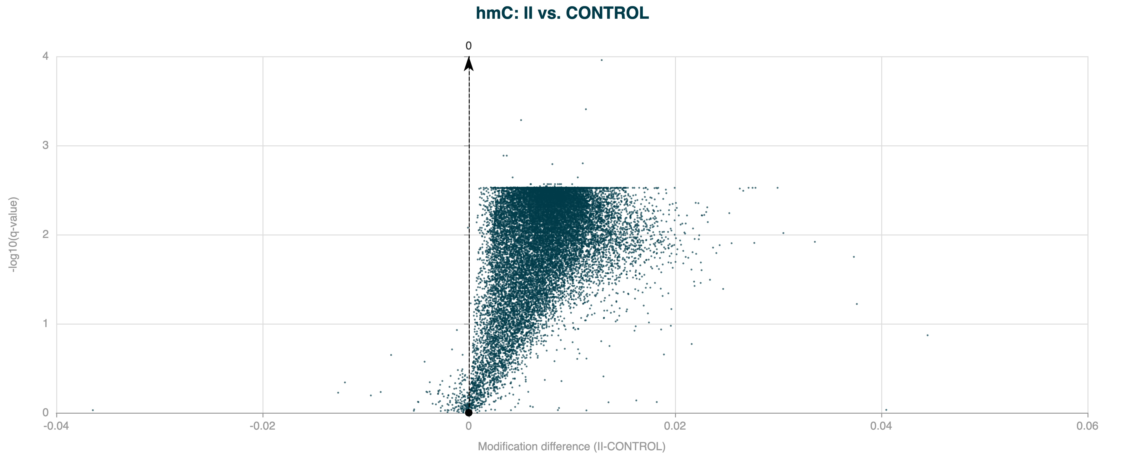
Figure 4 Volcano plot for 5hmC DMRs on gene bodies between Healthy Control and Stage II CRC cfDNA, showing many DMRs with similar q-values (plateau) after Benjamini-Hochberg correction.

Here’s a breakdown of how the BH correction works and why multiple DMRs can have the same q-value:

Suppose we have m tests with raw p-values p1, p2, ... , pm:

1. First step of the BH is to sort them in ascending order, so that p_sorted_1<p_sorted_2<...<p_sorted_m.

2. Each sorted p-value gets a rank i. The smallest p-value has rank 1, the highest has rank m.

3. The raw q-values are computed as q_i = (p_sorted_i * m / rank_i).

4. Crucially, the BH procedure forces that q-values are always increased with rank: to do that, replace each q-value with the minimum of itself and all q-values ranked below it.

Here’s how that might look in the data:

Rank	Test	p-value	Raw q-value	Adjusted q-value
1	A	0.0015	0.00750	0.00700
2	D	0.0028	0.00700	0.00700
3	E	0.0060	0.01000	0.01000
4	C	0.0250	0.03125	0.03125
5	B	0.0350	0.03500	0.03500

Notice how A has the lowest p-value, but the second lowest raw q-value? Therefore, the final step insures that the adjusted q-value of A is not higher than that of D by setting it to D.

This is not a bug, nor it is a problem - it’s what the BH correction does, which remains one of the most commonly used and most robust corrections available. This effect most likely arises when there are a lot of very small p-values. Therefore, it’s not surprising to observe this effect for gene-wide (i.e. very large region) p-values. Overdispersion correction can help mitigate this effect, but may not remove it completely. See Overdispersion correction for more details.

Overdispersion correction

When calling DMRs, the modality dmr call tool can apply an overdispersion correction to the statistical model.

When calling DMRs, the modality dmr call tool uses a logistic regression model to compare methylation levels between groups, assuming that methylation counts follow a binomial distribution (i.e., the variance is determined by the mean). The aim is to test the null hypothesis i.e., that there is no difference in 5mc, 5hmC, or modC methylation between the groups.

The comparison results in a p-value for any difference. A p-value tells you the likelihood that the difference being observed is due to random noise. The smaller the p-value, the more likely the difference is a genuine effect, and the null hypothesis can be rejected.

p-values hold values between 0 and 1 and when plotted, you would expect to see a flat distribution across most values but with a higher value close to 0. The peak close to 0 should represent a slight increase in frequency above the rest of the p-value distribution.

In real-world methylation data, the observed variance is often greater than expected under a simple binomial model due to biological and technical variability. This is called overdispersion, and can lead to increased levels of false positives, seen as a much higher peak close to 0 than expected. In the example below, DMR calling has been applied to human gene bodies, which are prone to overdispersion due to the large region size.

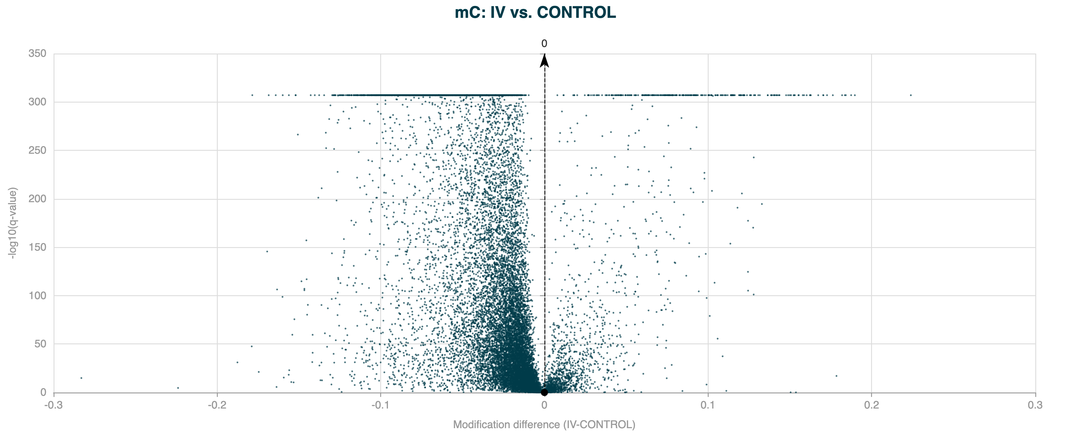
Figure 5 Volcano plot for 5hmC DMR results for human gene bodies, without overdispersion correction applied.

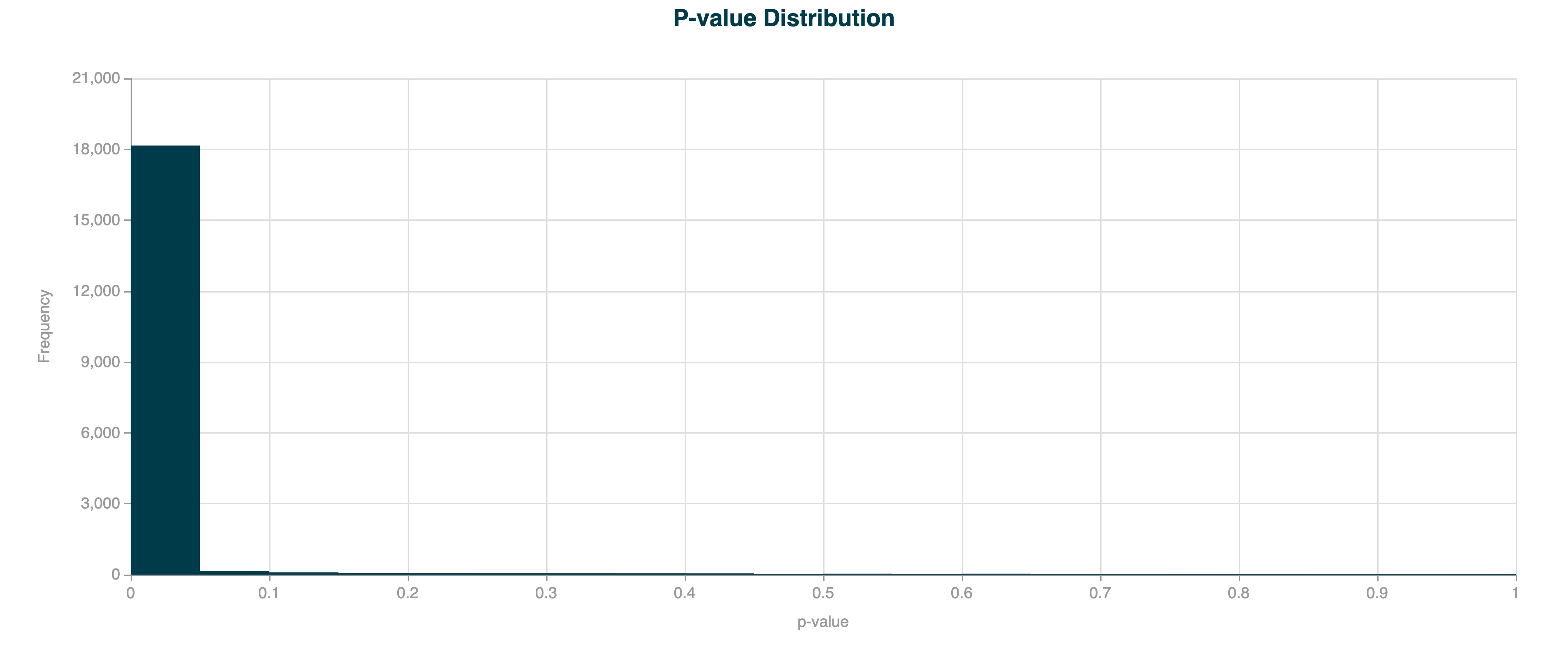
Figure 6 p-value distribution for 5hmC DMR results for human gene bodies, without overdispersion correction applied.

When --overdispersion is enabled, the model estimates an additional dispersion parameter (φ) for each region, following the approach of McCullagh and Nelder (1989, Generalised Linear Models, Chapter 4.5). This parameter adjusts the standard errors of the regression coefficients. The Wald test statistic and p-values are then computed using these adjusted standard errors, providing more accurate significance estimates. In the example below, the DMR calling has been applied to the same human gene bodies, but with overdispersion correction applied.

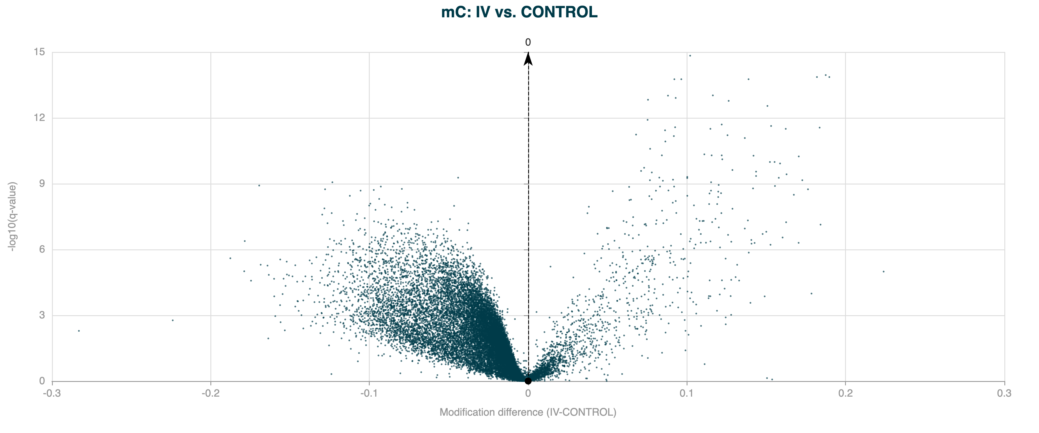
Figure 7 Volcano plot for 5hmC DMR results for human gene bodies, with overdispersion correction applied.

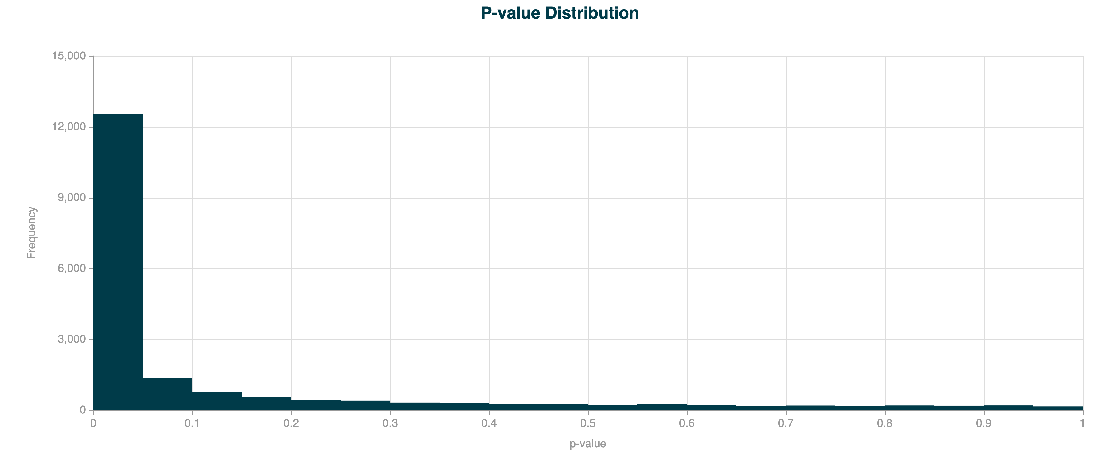
Figure 8 p-value distribution for 5hmC DMR results for human gene bodies, with overdispersion correction applied.

Without overdispersion correction, the model can underestimate the true variance, leading to inflated test statistics and an excess of false positives (i.e., regions incorrectly identified as significant). Overdispersion correction ensures that statistical inference is robust, especially when analysing large regions, heterogeneous samples, or data with technical noise.

You can diagnose the need for this option by inspecting the p-value histogram from your DMR results: a very sharp peak near zero suggests overdispersion is present and correction may be needed.

Sample size requirements for DMR analysis

We have implemented automatic sample size validation to prevent unreliable statistical inference in DMR calling. Logistic regression requires sufficient samples per group to estimate within-group variability - with too few samples (such as one sample per group), the model perfectly fits the limited data points but produces unreliable coefficients and artificially small standard errors, leading to meaningless p-values and increased false positive rates. Each group must have more samples than the number of model parameters (1 + number of optional covariates like age or batch) to ensure valid statistical inference - for example, with no additional covariates, each group needs at least 2 samples, increasing to 3 samples per group when adding one covariate. When insufficient samples are detected, the algorithm automatically skips the statistical test and returns conservative p-values of 1 and test statistics of 0 for all regions, effectively preventing false positives, and logs a warning message to inform users of the sample size limitation.

Users with insufficient samples can still examine the biological effect sizes by looking at the methylation differences between groups (mod_difference column) and fold changes (mod_fold_change column) in the results, which remain meaningful descriptive statistics even when statistical significance cannot be reliably assessed.

Calling DMRs

modality dmr call identifies regions where differentiated methylation occurs between different experimental groups. Examples of these groups are disease and normal, treated or un-treated or time-course experiments. A DMR is a defined genomic region where summed CpG sites show statistically significant differences in methylation between groups. Analyses may be scanning the whole genome, divided into fixed windows, or focussed on specific annotated regions provided in BED format.

Inputs

modality dmr call requires the following inputs:

• Zarr store(s): Paths to each Zarr store to include in the analysis.

• Sample sheet: Path to the sample sheet file containing metadata about the sample groups, or covariates. Covariates can be continuous (integers or floats) or categorical (strings).

• Output directory (optional): Path to the output directory where the result files will be saved.

Command

DMR calling is invoked by typing modality dmr call into the CLI terminal. To display a list of permitted arguments in the terminal, enter:

modality dmr call --help

Typical usage example:

modality dmr call \
   --sample-sheet path/to/metadata.csv \
   --zarr-path path/to/your/data.zarrz \
   --condition-array-name disease_stage \
   --methylation-contexts mc hmc \
   --bedfile path/to/regions.bed \
   --output-dir path/to/output/directory

The following table describes the tool options:

OPTION	Required	Description
-ss, --sample-sheet	Yes	Path to a sample sheet file containing a column with the header sample_ids, listing sample IDs that match the sample IDs in the Zarr store, and a column defining the experimental groups specified with the --condition-array-name option. Additional --covariates columns can be specified in the sample sheet but are not required. e.g., path/to/your/metadata.csv e.g., path/to/your/metadata.tsv
-z, --zarr-path	Yes	One or more paths to Zarr files separated by spaces. e.g., path/to/your/data.zarrz
-cn, --condition-array-name	Yes	String for grouping samples by a variable in the sample sheet, for DMR calling. The --condition-array-name value must exactly match the sample sheet column header. e.g., disease_stage.
-mc, --methylation-contexts	Yes	String to specify the methylation contexts to be analysed. Multiple contexts can be specified by separating them with spaces. The available contexts are: mC, hmC, and modc. Default value is modc e.g., mc hmc
-w, --window-size	No	Integer to specify the window size for DMR analysis. This option is mutually exclusive with the --bedfile option. e.g., 1000
-v, --covariates	No	String to specify the covariates to be included in the analysis. Multiple covariates can be specified, which must match the column headers in the --sample-sheet metadata file. Use double quotes if the covariate name contains spaces. e.g., covariate1 "covariate two"
-b, --bedfile	No	Path to a BED file containing regions of interest for DMR analysis. Any columns included past Chromosome Start and End in your DMR results file. e.g., path/to/regions.tsv
-mcv, --min-coverage	No	Integer to specify the minimum context sequencing depth for filtering. Filters the positions if the mean coverage across all samples in each position is lower than the desired filter value. Applied before grouping by -cn. e.g., 10
-nc, --num-contexts	No	Integer to filter out regions with fewer than the specified number of contexts. Only regions with at least this many contexts will be included in the results. Default is 0 (no filtering). e.g., 5
-r, --region	No	String to restrict analysis to a specific genome region. Use the format chr or chr:<start>-<end>. The start and end positions are optional, and indices are zero-based and half-open. e.g., chr1 or chr1:1000-2000
-dsm, --disable-strand-merging	No	Flag to disable strand merging to retain separate CpG sites on opposite strands (default: False, strands are merged). e.g., --disable-strand-merging
-od, --overdispersion	No	Include this flag to turn ON the overdispersion model. e.g., --overdispersion
-co, --condition-order	No	This feature is optional but recommended. If provided, the first condition in the list will be used as the reference (control) condition for DMR analysis. All other conditions will be compared to this condition, and then compared to each other. If not provided, sample order will match the --sample-sheet. e.g., HEALTHY I IV
-otd, --output-dir	No	Option to specify a path to an output directory. If not specified, the default output path is to the current working directory. e.g., path/to/output/directory
-c, --compress	No	Option to specify whether to compress the DMR output file using gzip compression. Include this flag to turn ON compression.

For more information on strand merging, see the Merging CpG strands section.

Important

The --window-size and --bedfile options are mutually exclusive. You must specify either a window size for genome-wide tiling or provide a BED file with regions of interest for DMR analysis. If neither option is provided, the tool will default to a window size of 1000 base pairs.

Outputs

The modality dmr call tool generates the following outputs in the specified output directory:

1. DMR result files: BED files containing the identified DMRs for each group pair and methylation context specified. The DMRs are annotated with the following columns:

Column	Description
Chromosome	Contig name.
Start	Start position.
End	End position.
num_contexts	Number of contexts in the window or region.
mean_coverage	Mean coverage of the contexts in the window or region.
mean_mod_group_1	Mean methylation level for group 1 (e.g., control).
mean_mod_group_2	Mean methylation level for group 2 (e.g., condition).
mod_fold_change	Difference in methylation level between groups 1 and 2, where mean(group 2) / mean(group 1). Note: Specifying the --condition-order option will determine the positive (hyper-) and negative (hypo-) methylation status of the DMR.
mod_difference	Difference in methylation level between groups 1 and 2, where mean(group 2) - mean(group 1). Note: Specifying the --condition-order option will determine the positive (hyper-) and negative (hypo-) methylation status of the DMR.
test_statistic	The Wald test statistic associated with the p-value.
dmr_pvalue	The p-value of significance of the difference in methylation levels between the two groups.
dmr_qvalue	The FDR-corrected p-value.
Annotation	This is an optional column that would be carried over from your BED file if provided see --bedfile option for more details. There is no limit to how many columns are carried over.
Name	This is an optional column that would be carried over from your BED file if provided see --bedfile option for more details. There is no limit to how many columns are carried over.

The DMR result files are named according to the following convention:

• dmr_<group1>_<group2>_<context>_window_<window_size>bp.bed, or;

• dmr_<group1>_<group2>_<context>_bedfile.bed if a BED file is provided.

A DMR result file in BED3+ format will be generated per pairwise condition, per modification. For example, for a 6-base DMR analysis that includes both methylation contexts (mc and hmc), with a DMR sample sheet that contains three conditions (e.g. healthy, cancer_stage1, and cancer_stage4), six result BED files will be generated in the output directory.

Tip

Consider the use of --output-dir for efficient management of the output files.

2. .ini files:

.ini file(s) contain the parameters used for the analysis, including the paths to input files. The matched .ini files use the same naming convention as the DMR result files. There will be one .ini file per DMR result file.

The content of the .ini file can be changed, to control which plots are included when using modality tracks. This allows editing of figure titles, axis titles, and optimising the order of the plots for clear communication of your findings. Navigate to the 1. Auto-generated .ini file section for more details.

3. Provenance metadata:

JSON sidecar files containing metadata about the analysis, including the command used, timestamp, version, and system information. The provenance metadata files are named according to the following convention:

modality_metadata_<YYYYMMDD>_<HHMMSS>.json.

Analysis examples

Example 1: DMR analysis on a single Zarr dataset for specific regions of interest

modality dmr call \
   --sample-sheet path/to/metadata.csv \
   --zarr-path path/to/your/data.zarrz \
   --condition-array-name disease_stage \
   --methylation-contexts mc hmc \
   --bedfile path/to/regions.bed \
   --output-dir path/to/output/directory

Example 2: DMR analysis on a single Zarr dataset for genome-wide screening by window size

modality dmr call \
   --sample-sheet path/to/metadata.csv \
   --zarr-path path/to/your/data.zarrz \
   --condition-array-name disease_stage \
   --methylation-contexts mc hmc \
   --window-size 1000 \
   --output-dir path/to/output/directory

Plotting differentially methylated regions (DMRs)

The modality dmr plot tool generates visualisations to aid the interpretation of DMR analysis.

The visualisations are volcano plots and histograms of p-values for each DMR result file, providing insights into the significance and magnitude of methylation differences between groups. These visualisations are helpful for result filtering, identifying significant DMRs and assessing the overall quality of the analysis.

The outputs of dmr plot provide insights into:

• The relationship between methylation differences and statistical significance: Volcano Plots

• The distribution of p-values across all tested regions, as a QC for DMR calling: p-value Histograms

Note

For different experimental reasons, there can be a very high frequency of p-values close to ‘0’, if this is the case, refer to Overdispersion correction for additional details regarding the --overdispersion option available in modality dmr call.

Inputs

modality dmr plot requires the following inputs:

• DMR result file(s): Paths to the output(s) of the modality dmr call tool, in .bed format. These files contain the DMRs identified in the analysis.

• Output directory (recommended): Path to the output directory where the result files will be saved.

Command

The DMR visualisation tool is invoked by typing modality dmr plot into the CLI terminal. To display a list of permitted arguments in the terminal, enter:

modality dmr plot --help

Typical usage example:

modality dmr plot \
   --dmr-results path/to/dmr_results.bed \
   --filter-qvalue 0.05 \
   --filter-mod-difference 0.1 \
   --output-dir path/to/output/directory

The following table describes the tool options:

OPTION	Required	Description
-dr, --dmr-results	Yes	One or more paths to DMR result files. These files are generated by the modality dmr call tool. e.g., path/to/dmr_results.tsv
-fq, --filter-qvalue	No	Float to filter DMRs by q-value. Only DMRs with q-values ≤ the specified value will be included in the plots and filtered output. e.g., 0.05
-fm, --filter-mod-difference	No	Float to filter DMRs by modification difference. Only DMRs with absolute modification differences ≥ the specified value will be included in the plots and filtered output. e.g., 0.1
-otd, --output-dir	No	Directory to save the generated plots. If not specified, the default output path is the current working directory. e.g., path/to/output/directory

Outputs

The modality dmr plot tool generates an HTML report per DMR results file input, in the specified output directory. Each HTML report contains the following sections:

1. DMR summary table

• Confirms the two Group names included in the DMR analysis, and which is the designated Control group and Test group, for calculating the modification difference, and directionality of hypo- and hyper-methylation.

• Shows the total number of regions (or windows) tested (after depth filtering).

• Shows the mean context depth, of all regions (or windows) passing q-value and/or mod-difference filter, if applied.

• Shows the mean number of contexts in all regions (or windows) passing q-value and/or mod-difference filter, if applied.

• If filtering was applied, the table will also show the number (and %) of regions (or windows) passing q-value and/or mod-difference filter.

2. Volcano plot

• Visualise the relationship between methylation differences (x-axis) and log transformed statistical significance \(-\log_{10}(\text{q-value})\) (y-axis).

• DMRs are included based on the specified q-value and modification difference thresholds.

• If provided with a --bedfile with multiple values in the Annotation column, the volcano plot data points will be colour-coded and an Annotation legend will be shown on the plot. Note that input bedfile annotations are carried over to the DMR results file used for plotting.

• The volcano plot is interactive, allowing you to hover over points to see details about individual DMRs.

• The plot can be manipulated with embedded tools, such as zooming and panning, to focus on specific regions of interest.

• Use the chart tools to save the image as .png.

3. p-value histogram

• Shows the distribution of p-values across all tested regions.

• Provides an overview of the statistical significance of the results.

• Helps to assess the overall quality of the DMR calling process, namely the proportion of significant DMRs.

• If provided with a --bedfile with multiple values in the Annotation column, a stacked histogram will be shown together with a legend on the plot. Note that input bedfile annotations are carried over to the DMR results file used for plotting.

The output files are named according to the following convention:

• HTML report: <dmr_result_file>_volcano.html

Analysis examples

Example 1: Plotting DMR results with filters

modality dmr plot \
   --dmr-results path/to/dmr_results.bed \
   --filter-qvalue 0.05 \
   --filter-mod-difference 0.1 \
   --output-dir path/to/output

Example 2: Plotting multiple DMR result files

modality dmr plot \
   --dmr-results path/to/dmr1.bed path/to/dmr2.bed \
   --output-dir path/to/output

Generate genomic track plots

The modality tracks tool generates genomic track plots for visualising methylation data, differentially methylated regions (DMRs), and gene annotations. This tool uses an .ini configuration file to define the tracks to be plotted, allowing you to customise the visualisation according to their needs. The .ini file is viewed, modified or created in a standard text editor.

The outputs of modality tracks provide insights into:

• Methylation traces: Visualising methylation levels across genomic regions for individual samples or groups.

• Methylation differences: Highlighting differences in methylation levels between groups, specifically hyper- and hypo-methylation.

• DMR tracks: Displaying the location and significance of DMRs.

• Annotations: Adding biological context to the visualisation using GTF/GFF files.

These visualisations are essential for interpreting methylation data and understanding its biological relevance.

The modality tracks command will generate a single track plot (.png or .pdf) containing the individual tracks that are specified in the .ini file. The tracks in the track plot will appear in the order they are listed in the .ini file.

Inputs

modality tracks requires the following inputs:

• ini file: Path to the .ini file to be included in the analysis.

• Output directory (optional): Path to the output directory where the result files will be saved.

This section details the data held in the .ini file, how it is structured, and which fields are editable. Instructions for creating a specific new .ini file are provided and these can be saved for future use.

1. Auto-generated .ini file

An .ini file is automatically generated by the modality dmr call tool when DMRs are called and saved in the output directory --output-dir specified in the command.

The .ini file is divided into sections. A section is indicated by square brackets [ ], and is descriptive if the track type. The use of mc/hmc/modC is dependent on the type of DMR analysis that was run. The main sections are:

Section	The section purpose
[DEFAULT]	Settings for each of the tracks e.g. size,title
[mc/hmc/modc methylation trace]	Methylation trace track for 5mC, 5hmC, or modC
[mc/hmc/modc methylation diff]	Methylation difference track for 5mC, 5hmC, or modC
[dmr]	DMR bar track
[spacer]	Adds vertical space between tracks
[gene]	Annotation track
[x-axis]	x-axis configuration

Each of these sections has a set of components which are populated in the auto-generated .ini file.

An example .ini file, after running modality dmr call for hmc DMRs between two conditions, CONTROL and I (specified by the column header, label, in the sample sheet metadata file:)

     [DEFAULT]
width = 20
figure_title = CONTROL vs I - hmc DMRs
disable_strand_merging = False
min_coverage = 0

[mc methylation trace]
type = zarr_methylation_trace
zarr = path/to/data.zarrz
metadata = path/to/metadata.csv
ymin = 0
ymax = 1
height = 3
title = hmc fraction
modification_type = hmc
group = label
group_trace = True
group_points = True
group_names = CONTROL; I

[spacer]

[mc methylation diff]
type = methylation_diff
zarr = path/to/data.zarrz
metadata = path/to/metadata.csv
height = 3
title = hmc difference
modification_type = hmc
ymin = -0.6
ymax = 0.6
group = label
group_names = CONTROL; I

[spacer]

[dmr]
type = dmr_bar
title = DMR magnitude
file = path/to/DMR_hmc_CONTROL__I.bed
dmr_header_present = True
y_min = -0.5
y_max = 0.5
height = 2

[spacer]

;[gene]
;type = gtf_gff
;file = path/to/gencode.gff3.gz
;file_type = gff3
;title = gencode
;height = 2

[x-axis]

Note

The [gene] section is commented out with a semicolon at the start of the line, meaning that the gene annotation track will not be included in the plot. To include the gene annotation track, remove the semicolon at the start of the line and ensure that the file path and type are correct. You will need to ensure that the GTF/GFF file is available and correctly formatted for the track to be built successfully.

Note

Users can choose whether they want to use a GFF3 or GTF file for annotation. The default expects a GFF3 but to pass a GTF file instead, change from ;file_type = gff3 to ;file_type = gtf and exclude the semicolon “;”.

Each section has its own components, the next table explains the purpose of the component, which are required, default settings and where input is needed.

Details of [DEFAULT]

Component	Setting	Purpose
width	default: 20	Width of the figure in inches
figure_title	default: None	Title for the entire figure
disable_strand_merging	default: matches DMR call setting	Boolean flag to disable CpG strand merging across all methylation tracks
min_coverage	default: 0	Minimum coverage filter: removes positions with coverage < min_coverage from tracks. Note: fractions are calculated with built-in min_coverage=1, so 0-coverage positions are not plotted regardless of this setting.

Details of [mc/hmc/modc methylation trace]

Component	Setting	Purpose
type	required	Must be zarr_methylation_trace
zarr	required	Path to the Zarr store
metadata	required	Path to the sample metadata CSV or TSV
ymin	default: 0	Minimum value for y-axis
ymax	default: 1	Maximum value for y-axis
height	default: 3	Height of the track in inches
title	default: None	Title for the track
modification_type	required	mc, hmc or modc
group	default: None	Metadata column to group samples
group_trace	default: True	Plot group traces (True/False)
group_points	default: True	Plot individual sample points (True/False)
group_names	default: None	Semicolon-separated group names, e.g., I; II

Details of [mc/hmc/modc methylation diff]

Component	Setting	Purpose
type	required	Must be methylation_diff
zarr	required	Path to the Zarr store
metadata	required	Path to the sample metadata CSV or TSV
ymin	default: -0.6	Minimum value for y-axis
ymax	default: 0.6	Maximum value for y-axis
height	default: 3	Height of the track in inches
title	default: None	Title for the track
modification_type	required	mc, hmc or modc
group	default: None	Metadata column to group samples
group_names	default: None	Semicolon-separated group names, e.g., I; II

Details of [dmr]

Component	Setting	Purpose
type	required	Must be dmr_bar
title	default: None	Title for the DMR bar track
file	required	Path to the DMR BED file
dmr_header_present	default: TRUE	Whether the BED file has a header
ymin	default: -0.5	Minimum value for y-axis
ymax	default: 0.5	Maximum value for y-axis
height	default: 2	Height of the track in inches

Details of [gene]

Important

To enable the gene annotation track, remove the semicolon at the start of only the following lines in the .ini file, including in front of the [gene] section header. Ensure that the GTF/GFF file is available and correctly formatted for the track to be built successfully.

Component	Setting	Purpose
type	required	Must be gtf_gff
title	default: None	Title for the annotation track
file	required	Path to the GTF/GFF annotation file
file type	required	gtf or gff
height	default: 2	Height of the track in inches

Details of [spacer]

There are no parameters for this section, when between sections it adds a vertical space between the tracks.

Details of [x-axis]

This is used to configure the x-axis and typically remains empty to deliver the default settings.

2. Customising .ini files

The default modality tracks visual is auto-generated but it can be customised. Table A shows default settings and ranges for components that can be used and Table B focusses on modifications of the .ini file. Changes are made by opening the .ini file in a text editor, updating with the changes and saving the file.

Important

Remember to save the updated .ini file and its path.

Table A: Default ranges

Component	Default	Range/Notes
width	20	>0
figure_title	None	Any string
disable_strand_merging	False	True/False
min_coverage	0	>=0, track filtering (see Note)
ymin, y_min	0/-0.5/-0.6	Any float, typically -1 to 1
ymax, y_max	1/0.5/0.6	Any float, typically -1 to 1
height	2 or 3	>0
group_trace	True	True/False
group_points	True	True/False
group_names	None	Semicolon-separated, e.g., I; II
dmr_header_present	True	True/False

Note

Understanding min_coverage in tracks:

There are two distinct coverage thresholds in the methylation plotting pipeline:

1. Fraction calculation threshold (always min_coverage=1): When methylation fractions are computed (e.g., mc / total_c), positions with coverage < 1 are automatically set to NaN to avoid division by zero. This happens internally and cannot be changed.

2. Track filtering threshold (default min_coverage=0): This is the parameter you set in the .ini file. It filters positions AFTER fractions are calculated:

   • min_coverage=0 (default): No filtering - all positions are kept, including those with NaN fractions from 0 coverage (these appear as gaps in plots)

   • min_coverage=N: Removes positions where coverage < N before plotting

Example: If you set min_coverage=10, positions with coverage 0-9 will be removed from the plot. Positions with coverage ≥10 will be displayed with their methylation fraction values.

Table B: modifying the ``.ini`` file

Modification	How to modify
Add tracks (plots)	Copy and paste the section to duplicate the type of plot.
Remove tracks (plots)	Delete the section from the .ini file, or comment out the section by including ; before each line to be ignored.
Change axis limits	Adjust ymin, ymax,``y_min``, y_max`` for each section.
Change grouping	Set group and group_names to match the metadata columns and values.
Add gene annotation	Remove ;, e.g. change ;[gene] to [gene] and set file to valid GTF/GFF file.
Customise titles	Edit figure_title and title fields to meaningful experimental titles for clarity.
Adjust panel order	Rearrange the complete sections in the .ini file.
Use p-value	Set use_qvalues = False in the [dmr] section to use raw p-values instead of q-values.

3. Creating an .ini file from scratch

When neither the default nor modification options for .ini file deliver the format of results required, a specific .ini file can be built. Using the details above as guidance for required components, here are the steps to building an .ini file:

1. Open a plain text editor such as TextEdit or a code editor such as Visual Studio Code.

2. Define the sections remembering they need to be enclosed in square brackets [Section name].

3. Add the key-value pairs e.g. title=hmc difference. The key is the ‘title’ and the value is ‘hmc difference’. The key-value pairs are therefore the components and values required to create the plot required.

4. Save the file with an .ini extension (e.g., config.ini) and note the path for use with modality tracks.

Important

There are best practices when working with .ini files:

• Always check that the file paths are correct and accessible.

• Use consistent group names with the sample sheet.

• Consider the y-axis scale when comparing mC and hmC DMRs.

• Save custom .ini files to be able to re-use the format.

Command

The tracks visualisation tool is invoked by typing modality tracks into the CLI terminal. To display a list of permitted arguments in the terminal, enter:

modality tracks --help

Typical usage example:

modality tracks \
   --tracks-file path/to/config.ini \
   --region chr1:100000-200000 \
   --output-dir path/to/output

The following table describes the tool options:

OPTION	Required	Description
-tf, --tracks-file	Yes	Path to the track configuration file (.ini) that defines the tracks to be plotted. The .ini file is created by the modality dmr call tool or can be created manually. e.g., path/to/config.ini
-r, --region	Yes	Genomic region to plot. Use the format chr or chr:<start>-<end>. The start and end positions are optional, and indices are zero-based and half-open. e.g., chr1:100000-200000
-otd, --output-dir	No	Path to save the generated plot. The output file format is determined by the file extension (e.g., .png, .pdf). e.g., path/to/output/track_plot.png or path/to/output/track_plot.pdf
-if, --image-format	No	Format for the output image file. Options: ‘png’, ‘jpg’, ‘pdf’, ‘svg’. Default: ‘png’. e.g., png or pdf
-p, --padding	No	Integer to specify the number of base pairs to extend the region on either side. Effectively, to zoom out. e.g., 1000
-dsm, --disable-strand-merging	No	Flag to disable strand merging to retain separate CpG sites on opposite strands (default: False, strands are merged). e.g., --disable-strand-merging

For more information on strand merging, see the Merging CpG strands section.

Outputs

The modality tracks tool generates a genomic track plot in the specified output file format (e.g., .png or .pdf). The plot includes the following tracks, as defined in the configuration file:

1. Methylation trace:

• Visualise methylation levels across the specified genomic region.

• Grouped by sample condition, as defined in the metadata file.

2. Modification difference:

• Highlight differences in methylation levels between groups.

• Smoothed and raw differences are displayed.

The solid line in the methylation trace and methylation difference tracks provides a smoothed representation of the data for improved readability. Smoothing is performed using a coverage-weighted Gaussian kernel-based approach. The smoothing scale is adaptive based on the length and density of the region that is being plotted.

3. DMR track:

• Display the location and significance of DMRs.

• Positive and negative DMRs are colour-coded.

• Uses q-values by default.

4. Annotation:

• Add biological context using GTF/GFF files.

• Display gene names, exons, and other features.

The output file is named according to the specified path and file extension, e.g., track_plot.png.

Analysis examples

Example 1: Generating a track plot for a specific region

modality tracks \
   --tracks-file path/to/config.ini \
   --region chr1:100000-200000 \
   --output-dir path/to/output

Example 2: Adding padding to the genomic region

modality tracks \
   --tracks-file path/to/config.ini \
   --region chr1:100000-200000 \
   --padding 1000 \
   --output-dir path/to/output

Extracting methylation statistics

The modality get command is designed to extract methylation statistic summaries for genomic regions or windows, from methylation data stored in Zarr format, from the duet software. This analysis can be used for creating datasets for classification algorithms, modelling gene expression, and examining potential coverage or methylation biases. This tool supports four key statistical summaries under the modality get command:

The four subcommands provide a specific type of statistical analysis, enabling you to explore methylation patterns across genomic regions of interest. The modality get command serves two main purposes:

1. Extraction of methylation statistics into a tsv.gz file, enabling feature-set generation and downstream analysis.

2. Visualise methylation statistics in HTML reports, to explore the distribution, correlation and hierarchical clustering of methylation across regions.

A typical Feature Extraction workflow requires:

• Specified data input.

• Selection of a statistical operation and methylation context(s) of interest.

• Specified genomic region(s) of interest or fixed window size.

Which in turn provides:

• Summarised methylation data as tsv.gz.

• HTML reports with interactive plots that can be saved as .png, for mean and regional-frac subcommands.

The next three sections explain how to extract the DNA methylation statistics, create and interpret HTML visualisations for insight into patterns in DNA methylation.

Inputs

The modality get command requires the following inputs:

1. Zarr path: Path to the Zarr file(s) containing methylation data.

2. Fields: Type(s) of cytosine to extract. Allowed --fields vary by subcommand (count, sum, mean, and regional-frac).

3. Region definition: Either a BED3+ file defining multiple genomic regions of interest, a single specified region, or a window size for genome-wide analysis.

Note

Field values: See Zarr store section for more information about available field values.

Optional input files

Optional file inputs are determined by the analysis being carried out:

• A text file in BED3+ format, listing the specific region(s) of interest.

• A text file in CSV or TSV format, containing sample group or condition metadata.

Commands

The modality get command is invoked by typing modality get into the CLI terminal. The command format is modality get <subcommand> <OPTIONS>.

Subcommands

To display a list of permitted arguments for a specific subcommand, type:

modality get <subcommand> --help

# e.g., for the `mean` subcommand
modality get mean --help

# e.g., for the `count` subcommand
modality get count --help

# e.g., for the `sum` subcommand
modality get sum --help

# e.g., for the `regional-frac` subcommand
modality get regional-frac --help

Example usage:

This illustration shows the subcommand with instructions to:

• Bring in specific Zarr store and .bed files

• Identify the modifications of interest (--fields)

• Visualise the results in violin, pearson correlation and regional heatmap plots

• Save the output files (Data .tsv.gz and Visualisations .html) to a specific output folder

modality get regional-frac \
   --zarr-path path/to/data.zarrz \
   --bedfile path/to/regions.bed \
   --fields mc hmc \
   --heatmap \
   --output-dir path/to/output

Common options

The following table describes the common options available. Note that not all options are available for all subcommands:

OPTION	Required	Description
-z, --zarr-path	Yes	Path to the Zarr file(s) to be analysed. e.g., path/to/data.zarrz
-f, --fields	Yes	Type(s) of cytosine to extract. Note that mc is synonymous to num_mc in the Zarr store. Allowed fields vary by subcommand. e.g., modc, mc, hmc, total_c
-mcv, --min-coverage	No	Integer to specify the minimum context sequencing depth for filtering. Filters the positions if the mean coverage across all samples in each position is lower than the desired filter value. Applied before aggregation with --aggregate-by-group. e.g., 10
-nc, --num-contexts	No	Integer to filter out regions with fewer than the specified number of contexts. Only regions with at least this many contexts will be included in the results. Default is 0 (no filtering). e.g., 5
-b, --bedfile	No	Path to a BED file defining genomic regions of interest. Mutually exclusive with --window-size. e.g., path/to/regions.bed
-w, --window-size	No	Integer to specify the window size for analysis. Mutually exclusive with --bedfile. e.g., 1000
-r, --region	No	String to restrict analysis to a specific genome region. Use the format chr or chr:<start>-<end>. The start and end positions are optional, and indices are zero-based and half-open. e.g., chr1 or chr1:1000-2000
-ss, --sample-sheet	No	Path to a CSV file containing sample metadata. e.g., path/to/your/metadata.csv e.g., path/to/your/metadata.tsv
-ag, --aggregate-by- group	No	Optional group name for aggregation. Reduces the dataset by summing count values for samples within each group. This affects all downstream analysis (correlation, PCA, etc.). Use this for merging technical replicates or combining samples by condition. Requires --sample-sheet. Cannot be used with --order-by-group.
-og, --order-by-group	No	Column name in the sample sheet to use for ordering samples in plots. Samples will be sorted by this group for visual organisation only. Does not perform aggregation - all individual samples remain in the analysis. Requires --sample-sheet. Cannot be used with --aggregate-by-group.
-hm, --heatmap	No	Flag to include a regional heatmap in the HTML report. Only available for regional-frac and mean. Drawing of the heatmap is limited to 200 regions. Default: FALSE.
-otd, --output-dir	No	Directory to save the output files. Default: current working directory. e.g., path/to/output
-cs, --case-sensitive	No	Flag to turn ON case-sensitivity for --aggregate-by-group and --order-by-group labels in the --sample-sheet. This option will preserve letter casing for label values. Default: FALSE. e.g., --case-sensitive
-t, --tabix	No	Compress output files using bgzip and create Tabix index. Requires installation of non-python dependencies (see Non-python dependencies). e.g., --tabix
-dsm, --disable-strand-merging.	No	Flag to disable strand merging to retain separate CpG sites on opposite strands (default: False, strands are merged). e.g., --disable-strand-merging

For more information on strand merging, see the Merging CpG strands section.

HTML report visualisations

Important

The HTML report is generated with get mean and get regional-frac commands, containing violin and Pearson correlation plots for each modification type 5mC, 5hmC, 5modC. If specified, a regional heatmap is also included for regional-frac and mean.

Plotting is not supported for count and sum subcommands, as these operations do not produce meaningful visualisations.

HTML files include multiple plots, with tools for performing basic manipulations such as saving the image in PNG format. A description of supported plots is provided below:

• Violin: A violin plot visually represents the density of data across a range of values. It will show DNA modification distribution across the DNA region. The violin also includes box and whisker plots.

• Correlation: A Pearson correlation matrix plot which visualises the relationship between two or more variables. It does not show causality. The deeper the colour the higher the correlation.

• Regional heatmap: A heatmap visualising the correlation and heirarchical clustering of methylation profiles across genomic regions and samples.

Optimising plots

1. Plotting subsets of samples

When working with a large number of samples, it may be useful to restrict the plotting to specific samples or group the analysis output based on sample labels. This may be for speed or where some samples have a specific biological element that is of interest.

The following options apply to plotting functions:

• --aggregate-by-group: Aggregates samples based on a common ID or group name column in the --sample-sheet where group labels are listed e.g. control or condition 1, treated or untreated, healthy or disease stage 1, etc. This action will reduce output results files and plots.

• --order-by-group: Orders samples based on a specific column in the --sample-sheet where group labels are listed. This action will not aggregate samples but will order them on the plot axes for easier visual interpretation. Result files are not reduced.

• --case-sensitive: This option allows for case-sensitive group labels, negating the default behaviour of converting group labels to uppercase in plots (see below).

2. Group labels

For plotting, the group label values are converted to uppercase by default. For example, Healthy and healthy would be assigned to the same group, HEALTHY. To override this behaviour, use the --case-sensitive option to report Healthy and healthy as separate groups.

Outputs

According to the modality get subcommand and analysis performed, the software shall return the following result files to the output directory. If an --output-dir path is not provided, the result files shall be saved in the current working directory:

1. Compressed TSV result file(s):

• Contains the extracted statistics for each genomic region.

• Columns include genomic coordinates, extracted values, and additional metadata in BED format.

• The file name is based on the subcommand used, e.g., <methylation-context>_<subcommand>.tsv.gz.

2. HTML report:

• Visualise the extracted statistics.

• Saved in the specified output directory as HTML files.

3. Provenance metadata:

• JSON sidecar files containing metadata about the analysis, including the command used, timestamp, version, and system information.

• The provenance metadata files are named according to the following convention: modality_metadata_<YYYYMMDD>_<HHMMSS>.json.

• The metadata includes the command used, timestamp, version, and system information.

Analysis examples

Example 1: Counting CpGs in genomic regions

This operation counts the number of CpGs in each region with a specific --fields modification status. It can also be used in conjunction with a minimum coverage setting.

modality get count \
   --zarr-path path/to/data.zarrz \
   --bedfile path/to/regions.bed \
   --fields total_c \
   --output-dir path/to/output

Example 2: Summing methylation counts across regions

This operation sums the total number of the selected --fields modifications across each region.

modality get sum \
   --zarr-path path/to/data.zarrz \
   --bedfile path/to/regions.bed \
   --fields mc \
   --output-dir path/to/output

Example 3: Calculating mean context value in each region

This operation can be used to assess the average coverage per CpG. For example, average number of CpGs covered at a specific depth in sequencing (total), or with a cytosine basecall (total_c).

modality get mean \
   --zarr-path path/to/data.zarrz \
   --bedfile path/to/regions.bed \
   --fields total_c \
   --output-dir path/to/output

Example 4: Computing regional methylation fraction over total_c

This operation is suitable for methylation fraction analysis and will calculate the proportion of a --fields out of the total number of unmodified and modified Cs (total_c), for each genomic region or window.

modality get regional-frac \
   --zarr-path path/to/data.zarrz \
   --bedfile path/to/regions.bed \
   --fields mc hmc \
   --heatmap \
   --output-dir path/to/output

Audit trail

Terminal feedback

modality XPLR provides immediate feedback in the terminal when commands are executed, showing:

• The command being run with all specified parameters

• Progress indicators for long-running operations

• Confirmation of output file creation

• Summary information upon successful completion

This feedback helps to confirm the command was interpreted correctly and analysis progression is being tracked.

Below is an example of the terminal output and provenance feedback generated during a typical modality biological-qc run:

2025-06-19 12:15:19  Provenance information:
2025-06-19 12:15:19  cmd='path/to/env/bin/modality biological-qc --zarr-path path/to/data.zarrz'
timestamp=2025-06-19T12:15:17.997570
version=1.0.0
user=user_name

2025-06-19 12:15:19  Running biological QC analysis:
2025-06-19 12:15:19  Zarr path(s): ['path/to/data.zarrz']
2025-06-19 12:15:19  Region: None
2025-06-19 12:15:19  Sample Sheet: None
2025-06-19 12:15:19  Group Name: None
2025-06-19 12:15:19  Output Dir: path/to/output

2025-06-19 12:16:27 | WARNING | path/to/env/lib/python3.x/site-packages/dask/core.py:127: RuntimeWarning: invalid value encountered in divide
return func(*(_execute_task(a, cache) for a in args))

2025-06-19 12:16:49 | WARNING | path/to/env/lib/python3.x/site-packages/dask/core.py:127: RuntimeWarning: invalid value encountered in divide
return func(*(_execute_task(a, cache) for a in args))

2025-06-19 12:16:55  Biological QC report generated: path/to/output/BioQC_YYYYMMDD_HHMMSS/biological_qc_report_<n>_samples_YYYYMMDD_HHMMSS.html
2025-06-19 12:16:55  Wrote provenance sidecar file to path/to/output/BioQC_YYYYMMDD_HHMMSS/modality_metadata_YYYYMMDD_HHMMSS.json

Logging and provenance tracking

Logs for every CLI command are written to a file named modality_cli.log in the current working directory for further inspection. Logging provides a record of events during the execution of modality XPLR commands. It helps to:

• Debug issues by reviewing detailed logs.

• Monitor the progress of long-running commands.

• Maintain a history of executed commands for reproducibility.

Provenance tracking ensures that every analysis is traceable by recording:

• The command executed.

• The timestamp of execution.

• The working directory and user.

• The version of modality XPLR used.

• System information (e.g., OS, Python version).

• A list of output files generated.

This metadata is critical for reproducibility and for understanding the context of results.

Process

• Provenance metadata: Captured automatically for every command.

• Output registration: All output files are registered and tracked.

• Sidecar file: Provenance metadata is saved in a JSON sidecar file alongside outputs.

• File comments: Metadata can be embedded as comments in output files (e.g. BED files).

For example, provenance metadata includes:

• Command: modality dmr –sample-sheet metadata.tsv –zarr-path file.zarr

• Timestamp: 2025-05-20T12:00:00

• modality XPLR version: 1.0.0

• User: first_name.last_name

• System info: { “os”: “macOS”, “python_version”: “3.11” }

• Outputs: [ “path/to/output/dmr_results.bed” ]

Provenance data is written to a JSON sidecar file in the output directory. A timestamp is included in the filename. e.g. modality_metadata_<YYYYMMDD>_<HHMMSS>.json

For CLI commands that produce BED format result files, the provenance metadata can be embedded as comment header lines in the output file.

Setting verbosity levels

How to set verbosity levels

The verbosity level in modality commands controls the amount of information displayed in the terminal during execution. This feature is useful for debugging, monitoring progress, or reducing unnecessary output.

modality XPLR supports three verbosity levels:

1. Default (no flag): Displays warnings and errors and command feedback only.

2. Information: Use --verbose or -v to display informational messages, warnings, and errors.

3. Debug: Use -vv to display detailed debugging information, along with informational messages, warnings, and errors.

To set the verbosity level, use the --verbose, -v (Information) or -vv (Debug) flags when running a modality command. The flag must be placed after the command and before any other options.

Each additional v increases the verbosity level. For example:

modality -v biological-qc \
   --zarr-path path/to/data.zarrz \
   --output-dir path/to/output/directory

modality -vv get regional-frac \
   --zarr-path path/to/data.zarrz \
   --fields mc hmc \
   --bedfile path/to/regions.bed \

This tool is particularly useful for monitoring long-running commands such as modality dmr call. Setting the verbosity level to Information will display progress bars, helping you to understand how far along the process is and if any issues arise. Below is an example of the terminal output when running modality -v dmr call:

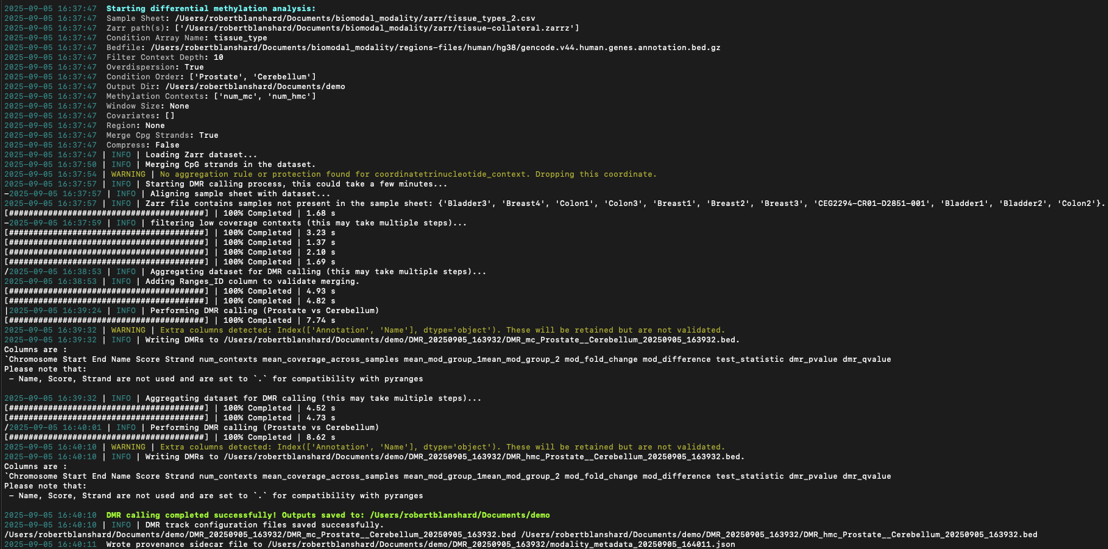
Figure 9 Terminal output showing progress bars for modality -v dmr call command.